Bilevel Optimisation for Equitable Wood Harvesting

Abstract

Malawians' dependence on forest products and agricultural demands have led to detrimental levels of deforestations. Their primary use of wood products is wood fuel for heating and cooking, although the government would prefer citizens switch to alternatives, the majority of people cannot afford other sources of fuel. Customary lands were the first forested areas to feel the effects of deforestation; now that they are depleted rural villagers are turning to government land- forest reserves. The government of Malawi introduced community based systems to include villagers in sharing the responsibility of combatting deforestation. A case study is performed using villages left of the Namizimu Forest Reserve; leaders from each village come together to form a committee that allocates trees to villages with the intention of avoiding over harvesting. Bilevel optimisation is applied to support the leaders in allocating wood fairly. Bilevel optimisation models the competing objectives of two parties. In this case, the committee wants to satisfy all villages equally, and the independent villages want to satisfy their own welfare. Although their goals are similar they create competition amongst the different parties. Bilevel optimisation removes any favourability from the allocation of wood, ensuring a more equitable division of supply. When there are few villages involved in the system we can solve for optimality. But if there are many villages, a heuristic may need to be designed to find a near optimal feasible allocation outcome. Equitable allocation is not enough for Malawi to reverse deforestation, proactive approaches to growing a more bountiful supply and behavioural changes need to be enacted.

1. Introduction

African miombo woodlands are disappearing due to substandard forest management practices influenced by demanding agricultural consumption, and dependance on wood products for income (Mwase et al., 2006). These harmful anthropogenic practices are forming a negative causal loop detrimental to both biodiversity and economic income of rural dwellers. Of the forested areas, customary woodlands (lands owned by indigenous people) are the most indisposed and devoid of forest management techniques. Rural Malawians primarily depend on customary lands and forest reserves for subsistence agriculture and wood products to support their livelihoods at the expense of the forests. In 2019, Malawi had a population of 18.6 million, by 2038 the World Bank expects the population to double. Heightened demand is clearing out customary lands, and people are desperately turning to forest reserves as their main source of supply, also threatening it. With rapid population growth, Malawi's problems are expected to worsen (World Bank, 2020).

Rural dwellers rely on forest products to support their own needs as well as to provide economic welfare by converting wood into fuel (firewood and charcoal) and cutting timber for construction, both of which they then sell to urban residents (Campbell, pg 2, World Bank, 2020). Income from forest products makes up approximately 15% of the average rural household's total income, preventing poverty and improving quality of life (Kamanga et al., 2009, Fisher 2004). Moreover, households whose incomes depend on forest resources the most are those that have little coming in from other sources, because there are not many other options for income (Chilongo, 2014, World Bank, 2020). The competing needs of food, income and fuel create a complicated and unsustainable relationship with the forest- subsistence farming negates the potential for economic welfare and vice versa.

Approximately 89% of all Malawian households do not have electricity, and 97% rely on some form of wood fuel to meet their energy related needs for cooking and heating. With charcoal and firewood being the most popular forms of wood fuel. Although the government is attempting to transition citizens to using other forms of fuel approximately 54% of urban households still rely on charcoal, because it is the cheapest option and they cannot afford other sources (Reytar, 2017). The second most popular wood product is timber. International demand for hardwoods have been profitable for Malawians who have few income alternatives.

Villagers initially harvested wood to support subsistence living, but now do so illegally and unsustainably for retail (Africa Geographic, 2019). It is predicted that demand for wood products will surpass supply by 2030, creating a shortage that will drive up prices for firewood and charcoal, leading to increased economic hardship for poorer urban residence who are unable to afford the elevated prices (Ministry of Natural Resources, 2017, pg 6). Through the international markets for forest products there has been increased economic activity, and Malawi has seen year over year growth within recent years, but it is still one of the poorest countries in the world (World Bank, 2020).

1.1 Deforestation

According to the FOA (Food and Agriculture Organization of the United Nations) (2020) global deforestation peaked in the 1990s when approximately 16 million hectares of forestry was lost each year (Houghton, pg 313, 2016). At the turn of the century this rate tapered and by 2015 to 2020 it was estimated at 10 million hectares per year, falling 37.5% from the previous decade. Currently, the FOA (2020) estimates global forestry covers 4.06 billion hectares, implying a 0.25% loss rate this year with expected year over year growth. The size of Malawi's total forested areas is currently unknown as forest management data has not been collected in almost two decades. The last reliable estimate was in 2001, at 2.6 million hectares of forests, covering 27.6% of the nation. Deforestation rates are estimated between 1-3%, occurring at 33,000 hectares a year- at least four times higher than the global rate (FOA, 2016, Ngwira & Watanabe, 2019).

Deforestation is known to negatively affect animal habitat, climate, and quality of soil to name a few. Global climate is impacted by deforestation when carbon stored within plants are released and earth's surface is physically altered. Deforestations warms the atmosphere by 1) adding the carbon stored in trees into the atmosphere 2) lowering the quantity of water in the evapotranspiration process, and 3) decreasing the overall amount of trees which can store carbon (Bala et al, 2007). Hajabbasi et al (1997) found that deforestation was harmful to soil, lowering its overall quality. Their research concluded that soil in deforested lands (compared to virgin forests) were 20% more compact, had 50% less nitrogen, and organic matter and soluble ions dropped by 10 to 15%. Research has also been done to understand the affects on large mammals' habitat. Kinnaird et al (2003) state many large animals prefer to remain a buffer of 2 to 3 kilometres away from forest edges. Therefore as forests continue to shrink so do habitats.

1.2 Problem

We demonstrate the use of bilevel optimisation for forest management, which to our knowledge has not yet been used. Although many strides have been made within the field, most research is focused on a single harvester and do not consider the competition of wood resources. From our research completed it has become clear that operational research methods have not been a predominant tool for battling deforesting in Africa. Malawi's deforestation crisis is both an environmental and socioeconomic issue affecting the livelihood of many citizens, placing urgency on this research. The proposed bilevel model is intended to support Malawi's government and community leaders in allocating wood for harvesting to villagers who may use wood products for personal use and/or for income.

The committee, consisting of community leaders, must consider the wood demands of each village and the distance they must travel to retrieve it. Each village is an independent actor, and may choose to do what is economically best for them rather than what is best for the environment. Their decisions will then affect the decisions of any other villages who choose to act after them. Wood cut from areas allocated to the village is considered legal, wood cut from any other area is considered illegal. Each village has its own objective function measuring economic welfare that it wants to maximise, and the committee's objective is a summation of all the villages less a penalty for wood allocated beyond minimum demand.

The allocation of wood to multiple villagers who are competing for resources resembles a Stackelberg-Nash game. The models seeks to emulate the behaviours of all participants:

Leader's allocation of wood for harvest - community leaders allocate wood with the intent of meeting villagers' demands, and discouraging any illegal harvesting. All supply can be allocated to further help avoid illegal harvesting, but that would defeat the purpose of protecting the forests from deforestation, so we penalise the leader for allocating wood beyond minimum demand with the intent of understanding the changes of allocation behaviour depending on the penalty.
Villagers' behaviours depending on fine for illegal harvesting and travel costs - each village wants to maximise their own welfare, but we would like to understand when the cost-benefit is worth it. Are travel costs worth the additional wood? Is risking paying a fine worth cutting wood illegally?
Influence of altruism on villages - Not all decision-making is financially influenced. We want to understand how altruism towards other villages and caring about conserving the environment will influence villagers' decision-making.

Although it is the responsibility of both the government and citizens to protect the forests, transitioning to a sustainable forest management program can appear exclusively beneficial in the long term triggering adverse behaviours in citizens who are suffering financially. This issue is not unique to Malawi, as it also occurs in many other African countries, such as Central Africa Republic, Zambia, and Democratic Republic of Congo to name a few (World Wildlife Fund). According to the World Economic Forum there are 60 million+ hectares of tropical forests on continental Africa, accounting for approximately 15-18% of the world's tropical forests with the second largest forest in the world being the Congo Basin. This model, 'Bilevel Optimisation for Equitable Wood Harvesting' is generalised, so it may be adapted to individual areas so that it is helpful to other areas and not just those villages in our case study- east of the Namizimu Forest Reserve.

Notable novelties of this work are:

A modelled Nash equilibrium framework amongst villagers competing for wood resources
Use of bilevel optimisation for forest conservation where forest usage is studied at a household level
A new case study involving a Stackelberg-Nash game between community leaders and village households east of the Namizimu Forest Reserve.

2. Background

In Malawi, there are catastrophic secondary effects for the climate such as dwindling water supply (Ministry of Natural Resources,2017, pg 1). If Malawians continue along this trajectory of abusing their natural forests they are projected to be wiped from existence by 2079. The crisis has required the Government of Malawi (GoM) to use unconventional approaches to curb illegal logging. In 2016, army forces were stationed at the Dzalanyama Forest Reserve to defend the trees and prevent further deforestation (Africa Geographic, 2019). Simultaneously the GoM began developing the National Charcoal Strategy to not only reverse deforestation but to create sustainable and economically beneficial logging habits for its citizens (Ministry of Natural Resources,2017, pg 7).

For many decades the GoM has been struggling with deforestation, and the National Charcoal Strategy is not their first attempt at fixing it, but an iteration of past policies. In 1997, the GoM implemented the Forest Act to establish a sustainable process for charcoal- to legally produce charcoal the individual or company must receive a government licence and follow the guidelines within the forest management plan. Though well intentioned, their guidelines were not sufficient and the policy led to the banning of charcoal production in 1997, furthering forest mismanagement, illegal harvesting, and loss of revenue for the country because there were not identifiable or affordable charcoal alternatives for citizens (Forest Act 1997, 1997). Illegal charcoal production continued to grow. It was evident that trees collected were from forest reserves and that if new policies were not enacted this behaviour would continue unchanged (Zulu, 2010). In 2016, the National Forest Policy focused its efforts to "achieve sustainable selfsufficiency of firewood, charcoal and forest product and services" (Malawi Government, 2016). The policy's approach was less top down, and aimed to empower citizens to be a part of the change towards sustainable charcoal production and forest management. Moreover, it included promoting alternative cooking energy sources, and bettered law enforcement to reduce illegal harvesting. While these efforts created cultural improvements, the increased national demand for wood products has negated many past efforts.

2.1 Co-Management

In the National Charcoal Strategy 2017-2027 the Ministry of Natural Resources, Energy and Mining outlined seven inter-related pillars to undertake the issues of shrinking forests and rising demands for household fuel. This Masters dissertation aligns with Pillar 4: Strengthen Law Enforcement, "The objective of this pillar is to enhance enforcement of existing laws and regulations in order to reduce illegal wood harvesting and charcoal production and to create a market for sustainable wood and charcoal production," (Ministry of Mines, 2017).

In previous years, villages were permitted to cut trees from land specifically allotted to them by the government. Trees cut from anywhere else were considered to be cut illegally. If caught, villagers were expected to pay a fine determined by how much was cut. This centralised approach did not work well as it was difficult to monitor the forests due to the limitations of the government, and the long journey to the city meant no one went to pay the fine nor held accountable. The Government of Malawi adjusted their approach by introducing co-management policies(GoM, 1997). This concept transfers the governing responsibility from the government to committees; each committee is responsible for a subset of villages, a specified forest area and is managed by villagers belonging to those villages.

Jumbe and Angelsen (2007) researched the effectiveness of community-based management, and deduced households were more likely to participate in conservation efforts if they are highly dependent on the forest. Although, if households cannot afford the fee to participate they will not and will therefore harvest illegally. Separately, villagers are obedient to their tribe's chief, if many villagers belong to the main tribe, and the chief supports forest conservation it is more likely that the villagers will too.

2.2 Case Study: Namizimu Forest Reserve

Namizimu translates to 'the place of the spirits.' The Namizimu forest reserve is located in the Mangochi district of Malawi's southern region, straddling Mozambique on its north-east boarder and Lake Malawi on its western boarder (Figure 1). It is a mountainous region with an altitude ranging from five hundred to eighteen hundred meters, spanning 82,831 hectares. The forest reserve still remains largely untouched, but is beginning to feel the burden of human activity such as harvesting of wood for charcoal and timber to satiate urban civilisation's demand (Dreoni, 2020). The GoM has not initiated co-management policies in this region yet, but plans to introduce it when they begin the Shire River Basin Management Program (GoM, 2013). As co-management has not yet been implemented here, there is an opportunity to use optimisation techniques to distribute wood equitably.

The villages east of Namizimu forest reserve are the main focus; villages west of the reserve are also close to Lake Malawi. These west side villages depend on fish products for their main source of income and are therefore not as reliant or susceptible to the forest. Of the villages on the eastern sides, there are 110 within a five kilometre buffer of Namizimu Forest for whom comanagement policies will be implemented (Dreoni, 2020).

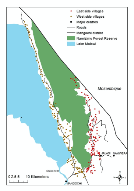
Figure 1: Image of the Namizimu Forest Reserve villages considered for this case study are in red.

3. Literature Review

Forest management optimisation models have evolved over the last 50 to 60 years where new techniques have emerged to utilise complicated non-linear relationships (Kaya et al., 2016). The field of forest management has arisen to meet ever growing human demand of forest products in a way that is less harmful towards the environment. Turner et al. (2002) acknowledge that environmental models contain unpredictable interactions between many elements making it difficult to model sustainability. To achieve modelling in the past, environmental problems were segmented into components of multiple simpler solvable models and then integrated with one another. But, with improved computing abilities and modern optimisation methods it has been possible to solve forest management problems with fewer but more intricate models.

Long-term sustainability is a challenge for forest management problems as there are frequently opposing objectives (Maser, 1994). Turner et al. (2002) use goal programming to find a strategy that satiates the competing objectives of the State Forests of New South Wales who are responsible for maintaining water, soil and biodiversity while fulfilling sawlog and pulpwood demands of local companies. A single level model was formulated to solve for the competing objectives, because although competing there was a sole decision-maker, which allowed for a single objective function to represent all decision variables. Data was not available for the intended 43 year planning horizon, and so final results are dependable for only the first 20 years. Results showed steady sawlog and pulpwood production could be achieved while upholding environmental responsibilities.

Bertomeu and Romero (2002) formulate and analyse the trade-off between tree biodiversity (age and species) and financial gain. Using a zero-one goal programming model they previously built, Bertomeu and Romero (2001) look to better understand and maintain the biodiversity forest stands (the quantity of trees in a woodland area). Their 2002 iteration develops the preceding harvest timetable's parametric constraints and gives insight into the opportunity cost for varying quantities of trees felled during harvest schedules. This model's graphs' visually capture the conflict between pay-offs clearly where other models have not.

Korhonen (1998) explores the application of Multiple Objective Linear Programming (MOLP) to forest management. In Multi-criteria Decision Making (MCDM) there are usually numerous criterium that must be satisfied to some degree to produce a set of options a decision-maker can select one from. Public forests supply communities with many products and services, and in this case study forrest management must decide how much of each should be supplied. Individual equations were written for each of management's eight goals and for the seven available forest resources effectively intertwining their relationships. Using a previously designed method by Korhonen and Wallenius (1998) called Pareto Race, which gives the decision-maker the ability to search along the boundary in their choice of direction and speed the MOLP was solved.

Saaty (1990) goes into detail about how to make a decision when multiple criteria needs to be considered. He developed the Analytical Hierarchy Process (AHP) to order factors in a top-down hierarchal format, layering objective, sub-criteria, and alternatives in descending order. Pair-wise comparisons are used to approximate the values of factors based on criteria until an outcome is established. Kuusipalo and Kangas (1994) apply AHP to a forest management problem, prioritising biodiversity and not just maximising economic output. Biological diversity is incorporated into the hierarchy's objective level and further elaborated and represented in the sub-criteria. The management strategies for whom revenue is of importance is placed in the hierarchy's lowest level. The strategy which best preserved biodiversity and brought in an acceptable profit was selected.

In recent years it has become popular to include carbon in the objective functions of forest management optimisation problems (Keles, 2010). Keles (2010) constructs three separate linear models for maximising the net present value of 1) harvested timber 2) carbon debt and 3) total carbon debt and timber produced. A simulation of the tree stands harvesting schedule is included. The combination of techniques concluded a 10.5% increase in net present value if the trees are cut no earlier than ten years of age.

Several authors have combined operational research techniques with economic utility functions to make better multi-criteria decisions. Utility functions quantify the satisfaction of consumer preferences by evaluating the utility gained from the consumption of goods (Chakrabati & Roy, 2010). Varma et al. (2000) built an aspiration-based utility function within a model using linear programming and geographic information systems (GIS). Using Mykkanen's (1994) approach for incorporating aspiration levels into utility functions the decision-makers preferences are demonstrated in the aspiration levels. Maximising the utility implicitly embodies the multicriteria partiality in attaining sustainability of temporal and spatial dimensions in forest management to propose strategies for the efficient use forest land. As the model seeks to address both current and future needs, it was pointed out that aspirations need to change as the times do.

Fürstenau et al. (2006) use multi-criteria analysis (MCA) to asses multiple purposes and stakeholders of an additive utility function for forest management alternatives. The various stakeholders are interested in the partial objectives- biodiversity, replenishing of ground water, quantity of timber and carbon sequestration which are prioritised using AHP. To understand how the climate and 6 forest management strategies will affect the forest over 100 years model 4C (Forest Ecosystems in a Changing Environment) is used. Model 4C simulates tree stands and the effects of 1) climate change on biodiversity, environment and forest growth, 2) ecological changes and 3) forest management strategies on the ecosystem (Lasch-Born et al., 2019). Utility for the six strategies were shaped by the priority of the partial objectives, i.e. strategies containing higher ranked partial objectives had higher utility.

Unlike the previously mentioned studies, Köhlin and Parks (2001) fight deforestation at a household level. Though many focus on forest management through companies and the government, deforestation is also highly impacted by the daily decision-making of millions of households relying on the forests for forest products (Köhlin and Parks, 2001). In India, one of the most successful strategies for decreasing deforestation was through implementing village woodlots for household fuel. A household utility function describes the collection behaviour of households who can choose between collecting fuel form natural forests, village woodlots and/or the market. The model is implicitly designed to maximise utility of decisions made by households. The method of Lagrange multipliers is used to find the optimum amounts of fuel wood collected at woodlots or natural forests and several other parameters. Results revealed decreased fuelwood harvesting in natural forests depends on the position of the village woodlot relative to the village and forest. The outcome is a non-linear upside-down 'U' that climaxes when village woodlots are approximately 3 kilometres from natural forests, indicating household decision making is most volatile here in respect to shadow wage.

Competing objectives or criteria may not always be beholden to a single decision-maker. Within Yeu and You's (2017) model decision-making is decentralised amongst two members of a biofuels and forestry supply chain- a harvesting company supplies forest products to a pulp company. The differences in their decision-making power can be deemed non-cooperative thereby aligning with a Stackelberg leader-follower game (von Stackelberg, 2011). Bard (1998) states bilevel programming problems (BLPP) can be viewed as a fixed form of von Stackelberg's leader-follower game. A follower's problem is generally limited to linear or quadratic programming; if binary parameters are included it creates a barrier to transforming the bilevel problem into a single level problem using Karusch-Kuhn- Tucker (KKT) conditions (Yeu and You, 2017). To overcome this obstruction Yeu and You (2017) use a reformulation-and- decomposition algorithm in place of KKT so they may include discrete variables for the follower in their mixed-integer bilevel problem. Both participants' objectives are to maximise their annual profit (annual revenue- total costs), by doing so the followers' decisions influence the leader's profit and decision space. The solutions showed that all members in the supply chain can earn up to 10% of revenue.

Although Yeu and You (2014) explore bilevel optimisation in relation to supply chain, a secondary market of forest management, the model addresses similar multi-criteria decisionmaking as equitable wood harvesting. The participants within this supply chain are a single leader and multiple followers, a Stackelberg-Nash equilibrium game. Stackelberg-Nash equilibrium game expands on Sackelberg game; the Nash equilibrium game simultaneously anticipates the outcome of decision strategies for several decision-makers where they all affect one another (Osborne and Rubinstien, 1994). Although there seems to be three levels of participants: suppliers, manufacturer and customers, suppliers and customers are group together as followers. The manufacturer (leader) which sits in the middle of the supply chain structure optimises for its own decision variables using a non-convex mixed integer nonlinear problem while the both lower-level customers and suppliers maximise their profits through optimising their activity in linear problems. A singular level was achieved through KKT reformulation, substituting the lower-level objective functions with KKT conditions. Global optimisation i.e. total profit for all participants was solved for using a branch-and-refine algorithm, with 80% of it belonging to the leader.

3.1 Social Games and Altruism

Batson (1943) describes altruism as "a desire to benefit someone else for his or her sake rather than one's own." Fehr and Schmidt (2005) state a person is altruistic if their utility raises in response to others' good fortune, or if \(\frac{\partial u}{\partial x}\) is strictly positive for u(x₁, x₂,..., x_N). Decision-makers within social games do not solely care about what is allocated to them, but also what is designated to others. This is unlike classical utility theories which state decision-makers seek to appease their own rational or conditions (Fehr & Schmidt, 2005). The decision-making process of followers within equitable wood harvesting encompasses their relative understanding of why their supply is limited to protect the environment and to ensure other villages have their needs met. This social responsibility can be measured using social games and altruistic utility functions. Even though every village may be aware of why their supply is limited it may not prevent them from acting selfishly; economic theories of Other-Regarding Preferences are utility functions that may explain the behaviours of the villagers. There are three subgroups of this theorem:

Social Preferences - players care about what the other players in the game are allocated.
Interdependent Preferences - players care about how altruistic or selfish other players are, and their preferences will sway to one the other depending on the other play.
Intention based Reciprocity - a player's preference will depend on what he thinks the other players' intentions are (Fehr & Schmidt, 2005).

Models categorised as social preference and interdependent preferences are explored. In some cases, players care more about their outcome relative to that of others more than they do about the amount itself, this is classified as relative income and envy (Bolton, 1991), a social preference. The model contains variables for how much is allocated to each player and their perceived value of their payouts during a specific period. Because \(\frac{\partial u}{\partial x} \leq 0\) it is the antithesis of altruism, it does not encompass unselfish behaviour (Bolton 1991).

Player i internally predetermine what quantity is an acceptable amount; if other players earn above that set amount player i will feel resentment towards them, but if they earn below it player i will feel altruism (Fehr and Schmidt, 1999). Player i has inequity aversion. Each player has a parameter representing their dislike for unfavourable inequality; player i is indifferent if they receive equal or more than player j, but will be dissatisfied if allocated less. This utility function requires heterogeneousness from players, and is able to justify the positivity and negativity of players towards others (Fehr and Schidt, 1999).

Quasi-maximin preferences blend Rawls' inequity aversion function, "disinterested social welfare function" with the sum of players' payoff to create a convex utility function, with the latter part representing altruism established on a concept of all players' payoffs are weighted equally. The utility function of each player is calculated through a mixture of the individual's payoff and the aforementioned function. Players are concerned about the welfare of others, but not as much if another player is more prosperous (Charness and Rabin, 2002).

One of the interdependent preferences utility functions is Levine (1998) altruism and spitefulness model. Each player is given a parameter ranging between selfishness to indifference to altruistic, and another for how much they care about the outlook of other players. Each player's goal is to maximise their utility either through their own success, that of others, or some combination of both. A downside to this model is that it cannot describe why a player may be spiteful in one instance but altruistic in another.

4. Methodology

Within Bilevel Optimisation there are two categories of competing decision-makers motived by self-interest. Each is represented by a level, level 1 or the upper level is modelled for the leader, and level 2 or the lower level is modelled for the followers which gives the decision making structure its bilevel. The followers constraints and objectives are a part of the leader's constraints, although the leader is influenced by the followers constraints the followers are not affected by the leader's. The equilibrium outcome from the lower level simultaneously influencing the performance of the objective function of the upper level ie the decisions of the lower level must be considered by the upper level if an optimal solution is to be found (Bard, 1998, Colson et al, 2007, Zeng & An, 2014).

Two strategic economic games are represented within this bilevel problem (BLP): Stackelberg competition and Nash equilibrium. The structure of the bilevel model captures the sequential decision making order of Stackelberg competition's leader first, follower after design. The original Stackelberg game had two players. The leader makes the first decision, which it cannot undo; and the leader is aware that the follower will be monitoring its actions. The leader is also privy to the decisions the follower will make in response. Whichever of the two players gains its position as the leader does so because they were already in an advantageous position. Although the leader has the advantage they must not abuse their power, because the follower has the option to refuse participation which will make the leaders plan infeasible (Dempe, 2002, Dempe et al, 2015).

If there is more than one follower, it can further be solved to find the Nash equilibrium amongst said followers. Nash equilibrium is a non-cooperative game consisting of 2 or more players, each player selfishly makes whichever decision they deem best for themselves, while knowing what was already decided for them by the leader (Osborne & Rubenstein, 1994). Each player's strategy will depend on events that have already occurred in the game. Therefore their strategy must change throughout the game in reaction to previous decisions made by opponents until their action is complete. The concluding cluster of strategy choices is considered a Nash equilibrium.

A Stackelberg-Nash game can be mathematically formulated as follows (Bard, 1998, Colson et al, 2007):

\(\max \limits_ {x \in X, y} \quad F(x,y)\)

\(s.t. \quad G_i (x,y) \leq 0 , \quad i= 1,..,n \)

\(\max\limits_y \quad f_k(x,y) \quad k=1,..l\)

\(s.t. \quad g_j (x,y) \leq 0, \quad j=1,..m\)

For equitable wood harvesting, the leader is a committee formed by a group of villages, and the followers are the villages. The committee's objective is to maximise welfare for the group of villages, to be successful the committee must maximise the welfare of each individual village. Welfare is quantified by calculating income from selling wood, cost of transportation, fine for illegally wood, other income, and a measure for altruism which is assumed to influence decision making.

Economic preferences and utility theory best represent welfare. Utility can be described as: \(u(x) \geq u(y) \, \Leftrightarrow \, x \succeq y\). A player chooses between x and y, if the utility of x is greater than the utility of y then x is 'weakly preferred' to y, that is y will not be selected over x when there is a choice to make between the two. By observing the choices players make the utility implicitly translates their values (Ingersoll, 2019). For villages, this structure is captured in their decisionmaking about legal and illegal wood, we can understand the value of each through utility. The value of each unit of wood is expected to decrease as each additional unit is acquired, therefore each unit is of lesser value than the previous one, the welfare function must therefore take on a concave shape.

The committee is tasked with allocating wood to villages in a manner that will satisfy their demands, the committee must also anticipate the villages making their own independent decisions. Despite having the ability to autonomously make decisions, each village may be influenced by the committee to some degree. They must decide if harvesting wood from elsewhere is worth the fine charged for illegal behaviour. This BLP consists of N villages, and 1 leader, therefore the model is solving for N+1 non-linear programming models simultaneously, capturing the intertwining relationship amongst the N+1 parties.

4.1 Altruism and Decision Making

It is assumed within a Nash equilibrium game all players are selfish therefore caring about only their own financial outcomes (Levine, 1998). But, economist such as Kenneth Arrow (1981) and Amartya Sen (1995) have alluded that not all people solely care for themselves, they also care about how their decision-making will affect others. Other economist expressed that people care mostly about fairness and for mutuality in social interactions (Fehr & Schmidt, 2005).

It was crucial to include an element of altruism in equitable wood harvesting. When interviewed, villagers in Malawi expressed that they understood the need for co-management schemes to protect the environment and to ensure that everyone gets their fair share of the supply (Dreoni, 2020). It also matters because if a single village chooses to maximise their own utility function it may grossly harm the other villages thereby leading to an overall low objective outcome for the leader. 'Theories of Other-Regarding Preferences' were previously explored in the Literature Review, concluding Levine's (1998) model for 'Altruism and Spitefulness': \(U_i = x_i +\sum_{j\neq i} x_j (\alpha_i + \lambda\alpha_j)/(1+\lambda)\) to be later adapted, was best suited to exemplify the relationship between villages.

Each village's utility function outcome is an average altruism score of their interrelationships with all the other villages in the game. Using \(\lambda\) we can quantify how much a village cares about the others opinions of altruism, though it may be counter intuitive, if a village is altruistic towards one that is spiteful (\(-\lambda\alpha_j > \alpha_i \)) village i will act more spitefully towards itself. If the utility function will shorten to \(U_i = x_i +\alpha_i\sum_{j\neq i}x_j\), this makes it possible (but not strictly) for i to have a higher utility score than if both i and j were included (\(\lambda > 0\) and \(\alpha_{i'} ≤ 0\)). Adding in this component to each village's objective function somewhat forces them to consider others as being too selfish will negatively impact their objective function.

4.2 Karush-Kuhn-Tucker Reformulation

Bilevel optimisation models are non-convex and non-differentiable. Jeroslow (1985) and Hensen et al (1992) independently demonstrated that bilevel problems are NP-hard even when in the simplest form of both upper and lower problems being linear (Colson et al., 2007). To solve BLPs the two levels can be reformulated into one level with complementarity constraints by using Karush- Kuhn- Tucker (KKT) optimality conditions, producing a computationally feasible problem. For KKT to be used, the lower level problems' objective function must be twice differentiable and not contain any discrete variables (Dempe, 2002).

KKT is derived from the method of Lagrangian multipliers which exclusively uses only equality constraints. For all villages we remove their individual optimisation models and replace them with their optimality conditions, each of the conditions will gain a unique Lagrangian multiplier for every village. These conditions will be treated as constraints for the BLP. KKT's theorem states, if a saddle point is found for Lagrangian function an optimal solution vector exists for the system. Although the Lagrangian function itself is not used, its first order differentials for x and y (lower level's decision variables) are used to establish stationarity which is an essential condition to solving KKT (Dempe, 2002).

For KKT to be solvable there are necessary conditions that must be satisfied 1) stationarity for the decision variables, 2) primal feasibility, 3) dual feasibility and 4) complementary slackness. If the conditions are fulfilled all optimal solutions will be among the KKT points, and it is possible to have more KKT points than optimal solutions, at minimum there will be sufficiency all KKT points will be a part of the optimal solution. Complimentary slackness is the product of a Lagrangian multiplier and lower level constraint all brought to the left hand side (slack) equal to 0; they are orthogonal meaning that one of them must be 0. The 'slack' equations are included in the Lagrangian function (to be differentiated for stationarity), if the slack is negative or zero it is feasible, if it is strictly positive it becomes a penalty. Furthermore, regularity conditions or constraint qualifications need to be satisfied for KKT to be used. For the BLP of equitable wood harvesting, all constraints are linear affine functions, so no additional conditions need to be satisfied (Dempe, 2002).

Once all conditions are met a global saddle point may be found in the cone of feasibility. The saddle point is the point where all the gradients for x (and y) orthogonally intersect and are equal to 0 thereby meeting the constraint \(\frac {\partial L} {\partial x} = 0\) (\(\frac {\partial L} {\partial y} = 0\)). If there is necessity (ie more KKT points than optimal solutions) each solution to this system of inequalities will become an optimum solution for each village and a solution to that system (Dempe, 2002).

Additionally, even if all conditions are satisfied bilevel problems are still difficult to solve in nature. This is because the Lagrangian and complementarity constraints contain non-convexities; and the complementarity constraints are inherently combinatorial (Colson et al, 2007). The complexities are BLP rapidly increase as N increases, which each value of N increase the model must consider an additional LP model. The solution space grows much larger and the time to computational solve the problem grows exponentially (Dempe, 2002).

4.3 High Point Relaxation

As mentioned above, the method of solving a BLP using KKT reformulation becomes complex quickly with each unit of N increase. Another approach for solving the BLP is to use high point relaxation, but unlike with KKT the solution does not converge towards optimality, but towards a feasible region. Because there are significantly less constraints and variables less computational time is required (Zeng & An, 2014).

High point relaxation solves the upper level problem and finds the optimum outcome for the leader; the lower level objective functions are dropped and constraints from both levels are kept. Though the leader's decision making is influenced by the constraints of the followers, the leader's decision still reflects their ideal solution, not a realistic one. It removes independent decision making power from the followers, and ignores that this is a non-cooperative game seeking an equilibrium (Zeng & An, 2014).

By using high point relaxation we can fix the quantities allocated to each village by the committee. This will provide critical insight into the decision-making strategies of the independent villages without any influence of the committees objective to maximise the overall welfare of all villages.

For equitable wood harvesting, the leader's decision variable is \(\overline x\), for the followers they are x and y. When the committee allocates wood to each village, it would undoubtedly prefer the villages strictly cut wood legally (x) and not illegally (y). Therefore it is necessary to solve the lower level programming model to understand the selfish motives of the villages who pursue maximising their own welfare.

4.4 Assumptions

All villages within the system will take part in the community based scheme, even though we already know that all villages do not take part. One of the limitations to using KKT conditions to reformulate bilevel problems is that discrete variables cannot be included in the lower problem, therefore we cannot use a binary variable to identify which villages are interested in having wood allocated or not.
Dreoni (2020) states fees for taking part in the scheme are relative to the quantity of demand and the tree type. For this model all trees are valued the same.
We assume that if distance to allocated supply is far a village may choose to go elsewhere instead to decrease their own costs.
All villages who cut wood illegally will pay the fine they owe. In reality, villages only pay the fine when they are caught cutting illegal wood and make the effort to go pay it. It is more likely that a villager may get away without paying the fine.
Behaviour to harvest illegally will be influenced by the altruism portion of the objective functions.
Villagers must carry wood roundtrip, that is, their journey begins at their village to a single supply of wood then back to the village, but if the truck is not full they could go to other areas of supply before returning to the village.
Personal demand is static. The figure used for minimum demand represents how much the village uses for themselves, and then all other wood harvested beyond that is for sale. But, a village can harvest more than minimum demand and not sell any of it.

4.5 Model

Parameters

i - the number of villages from 1,...,N

j - the number of disjointed woodland area resources 1,...,k

\(\delta\) - parameter weighting how much value the utility earned from the quantity of wood the village collects should be a part of overall welfare

\(\lambda\) - indicates how much a village cares about other villages' opinions on altruism

fee_i - cost to be included in allocation of wood for each village i

d_i - minimum units of wood demanded by each village i

s_j - units of wood supply in each woodland area j

distance_ij - distance between village i and woodland area j

WPT_i - units of wood village i can carry on each trip (wood per trip)

I_i - any other income the village i earns

\(\alpha_i\) - altruism score of village i

max_travel_i - the total maximum distance village i is capable of travelling for wood

SF - scalar factor for fee and Income

SP - scalar factor for fine

penalty - quantity the committee is penalised by for each unit of wood allocated beyond minimum demand

bigM - arbitrary parameter to bound variables without upper or lower limits

Constants

\(\gamma\) - cost of fuel per km

\(\beta\) - selling price per unit of wood

\(\phi\) - a fixed penalty fee for each unit of wood harvested by village i outside of its allotted j areas

Variables

\(\overline x_{ij}\) - units of wood allocated to village i in area j by the committee

\(x_{ij}\) - units of wood legally harvested by village i

\(y_{ij}\) - units of wood illegally harvested by village i

\(\eta_i, \theta_i, \mu_i, \nu_i,\xi_i, \pi_i, \zeta_i\) - Lagrangian multipliers for each village i

The objective function for the lower level calculates welfare for the individual villages within the community. Welfare is not a sole measure of economic welfare, but also includes altruism. The purpose of combining these two components is meant to understand their contentment with the overall community-based system, because the true virtue of this model is to support deforestation efforts while ensuring rural villagers can also survive. As it is the responsibility of the committee to ensure all villages receive equitable welfare based on their needs, the upper level's objective function is a summation of all the lower level objective functions. The objective function contains the following sub-equations:

Revenue: units of wood sold after the minimum demand is set aside for the village i's own use, legal or illegal acquisition of the wood is negligible.

\(h_1 (x,y, d) = 1- \) \(\exp ^{-\beta (\sum_j (x_{ij}+y_{ij}) - d_i) } \qquad \forall \, i \in N\) (1)

Travel Costs: the cost to travel the total distance (km) to retrieve the wood from area j and return to village i.

\(h_2 (x,y,d) = 1-\) \(\exp^{- \gamma \sum_j(\frac { (x_{ij}+ y_{ij})} {WPT_i} \times (2distance_{ij}))} \qquad \forall \, i \in N\) (2)

Altruism Score: the altruism score measures how happy villages are with the outcome of wood acquired by all villages, where village i has an altruism coefficient -1 < \(\alpha_i\) < 1. If \(\alpha_i\) > 0 the village is altruistic, if \(\alpha_i\) = 0 village i is selfish, otherwise spiteful. \(\lambda\) ranges 0 ≤ \(\lambda\) ≤ 1, it symbolises how much a village cares about being fair, the higher the value of \(\lambda\) the more a village is altruistic towards another who emotes mutually. The parameter \(\delta\) is used to test how behaviour changes when more or less importance is placed on utility gained from village i's own harvest.

\(h_3 (x,y, d) = \delta \frac {\sum_j (x_{ij} +y_{ij})} {d_i}\) \( + \frac {1} {N-1} \sum_{i \neq i'} (\frac {\sum_j (x_{i'j}+ y_{i'j})} { d_{i'}}\) \(( \frac {\alpha_i + \lambda \alpha_{i'}} {1+ \lambda} )) \qquad \forall \, i \in N\) (3)

Level 1

Objective Function

\(Maximise \quad\) \( \sum_i [h_1(x,y,d)\) \( - h_2(x,y,d)\) \( + h_3 (x,y,d)\) \( + SF(I_i-fee_i)\) \( - SP(\phi_i\) \(\sum_j y_{ij})\) \(- penalty(\sum_j \overline x_{ij} - d_i)]\) (4)

Constraints

Supply:- units of wood allocated to the sum of village i from woodland j cannot exceed the units of wood available at woodland j.

\(\sum_i \overline x_{ij} \leq s_j \qquad \forall \, j \in k\) (5)

Demand- the units of wood allocated to each village i should at least meet their minimum demand.

\(d_i \leq \sum_j \overline x_{ij} \quad \quad \forall \, i \in N \) (6)

Non-negativity- wood allocated from woodland j to village i cannot be less than zero.

\(\overline x_{ij} \geq 0 \quad \quad \forall \, i, j \in N,k\) (7)

Roundtrip Distance- each village i can afford to travel a max distance, woodland areas allocated to villages should take the distance into account.

\(\sum_j [ \frac {\overline x_{ij}} {WPT_i} \times 2distance_{ij}] \leq\) \( max \_ travel_i \quad \quad \forall \, i \in N\) (8)

Level 2

Objective Function

\(Maximise \quad h_1(x,y,d)\) \(- h_2(x,y,d)\) \(+ h_3 (x,y,d)\) \(+ I_i\) \(- SF(fee_i)\) \(- SP(\phi_i \times \sum_j y_{ij}) \quad \forall i \in N\) (9)

Constraints

Legal wood chopped- village i is permitted to cut no more than the allocated units of wood (\(\overline x_{ij}\)) from woodland j.

\(x_{ij} \leq \overline x_{ij} \quad \quad \forall \, i, j \in N, k\) (10)

Total wood Chopped by a Village- village i can decide where it would like to harvest wood from regardless of where and how much was allocated to them, wood harvested from anywhere other than \(\overline x_{ij}\) is considered illegal (\(y_{ij}\)). The decisions of village i will affect those of villages i'.

\( x_{ij} + y_{ij} \leq \) \(s_j\) \(- \sum_{i' \ne i}(x_{i'j} + y_{i'j})\) \( \qquad \forall \, i, j \in N, k\) (11)

Meeting Demand- village i may be satisfy their demand by harvesting wood legally and illegally, demand is elastic and may increase especially for those selling the excess beyond their subsistence needs.

\(d_i \leq \sum_j (x_{ij}+y_{ij}) \qquad \forall \, i \in N\) (12)

Distance Travelled- each village can only afford to travel a max distance, they may prefer to maximise their units of wood by harvesting from a closer location that many not have been allocated to them.

\(\sum_j [\frac {x_{ij}+ y_{ij}} {WPT_i} \times 2distance_{ij} ] \leq \) \(max\_travel_i \qquad \forall \, i \in n\) (13)

Supply Available- the units of wood harvested in woodland j cannot exceed supply.

\(\sum_i (x_{ij} + y_{ij}) \leq s_j \qquad \forall \, j \in k \) (14)

Non-negativity- a village cannot harvest negative units of wood.

\(- x_{ij} \ , - y_{ij} \leq 0 \qquad \forall \, i, j \in N, k\) (15)

Conditions for y_ij > 0village i must harvest the max amount of wood allocated to them before they cut any wood illegally in woodland j to maximise their objective function. This constraint is implied in the objective and does not need to be made explicit to solve.

\(y_{ij} > 0 \Leftrightarrow x_{ij} \geq \bar x_{ij}, \forall i \in [n], j \in [k])\) (16)

L2 Reformulation

\(Let \, L = L(x,y,d,\eta_i, \theta_i, \mu_i, \nu_i,\xi_i, \pi_i ) \) (17)

\(L=\) \(\sum_i (h_1(x,y,d)+ I \) \(- h_2(x,y,d) \) \(+ h_3(x,y,d) \) \(- SF(fee_i) \) \(- SP(\phi_i \times \sum_j y_{ij}) \)
\(- \eta_i ( \sum_j (x_{ij}) - \overline x_{ij}) \) \(- \theta_i \sum_j( x_{ij} + y_{ij} -s_j + \sum_{i'≠ i} (x_{i'j}+y_{i'j})) \) \(-\mu_i (d_i - \sum_j (x_{ij}+y_{ij})) \)
\(-\nu_i ( \sum_j [\frac {x_{ij}+ y_{ij}} {WPT_i} \times 2dist_{ij} ] - max\_travel_i) \) \(- \zeta_i \sum_j (x_{ij} +y_{ij} - s_j) \) \(+ \xi_i (\sum_jx_{ij}) \, \) \(+ \pi_i (\sum_jy_{ij}))\) (18)

Stationarity

The optimum units of legal and illegal wood to be harvested are given by:

\(\frac {\partial L} {\partial x} = \sum_i [\beta \exp ^{-\beta (x_{ij}+y_{ij} - d_i) } \) \(-(\gamma( \frac {2distance_{ij}} {WPT_i}) \exp^{- \gamma (\frac {x_{ij}+ y_{ij}} {WPT_i} \times 2distance_{ij})}) \) \(+ \delta ( \frac {1} {d_i} + \frac {1} {N-1} \sum_{i'≠i} \frac {1} {d_{i'}} ( \frac {\alpha_i + \alpha_{i'}} {1+\lambda} )) \) \(- \eta_i \) \(- (\theta_i + \sum_{i'} \theta_{i'} ) \) \(+ \mu_i \) \(- \nu_i(\sum_j \frac {2distance} {WPT_i}) \) \(- \zeta_i + \xi_i= 0 \)(19)

\(\frac {\partial L} {\partial y} = \sum_i [-\beta \exp ^{\beta (x_{ij}+y_{ij} - d_i) } \) \(-(\gamma( \frac {2distance_{ij}} {WPT_i}) \exp^{- \gamma (\frac {x_{ij}+ y_{ij}} {WPT_i} \times 2distance_{ij})}) \) \(+ \delta ( \frac {1} {d_i} + \frac {1} {N-1} \sum_{i'≠i} \frac {1} {d_{i'}} ( \frac {\alpha_i + \alpha_{i'}} {1+\lambda} )) \) \(- (SP* \phi) \) \(+ \theta_i \) \(- \sum_{i'} \theta_{i'} \) \(+ \mu_i \) \(- \nu_i ( \sum_j \frac {2distance} {WPT_i}) \) \(- \zeta_i + \pi_i = 0 \) (20)

Complementary Slackness

Legal wood chopped:

\(\eta_i ( \sum_j (x_{ij}- \overline x_{ij})) = 0 \qquad \forall i \, \in [n]\) (21)

Total wood Chopped by Village:

\(\theta_i ( x_{ij} - y_{ij} -s_j \) \(+ \sum_{i'≠ i} (x_{i'j}+y_{i'j}))= 0 \qquad \forall i \, \in [n]\) (22)

Demand:

\(\mu_i (d_i - \sum_j (x_{ij}+y_{ij})) = 0 \qquad \forall i \, \in [n]\) (23)

Distance:

\(\nu_i ( \sum_j [\frac {x_{ij}+ y_{ij}} {WPT_i} \times 2dist_{ij} ] \) \(- max\_travel_i) = 0 \qquad \forall i \, \in [n]\) (24)

Supply Available:

\(\zeta_i( \sum_i (x_{ij} + y_{ij}) - s_j= 0 \qquad \forall \, j \in k \) (25)

Non-negativity:

\(\zeta_i( \sum_i (x_{ij} + y_{ij}) - s_j= 0 \qquad \) \( \forall \, j \in k \) (26)

\( - \pi_i (y_{ij})= 0 \qquad \qquad \qquad \quad\) \( \forall i \, \in [n], j \in k\) (27)

\(\eta_i, \theta_i, \mu_i, \nu_i,\xi_i, \pi_i ≥ 0 \qquad \quad\) \( \forall i \, \in [n]\) (28)

4.6 Solving using Baron in AMPL IDE

Finding a solution to BLP relies on branch-and-bound techniques (Zeng & An, 2014); to solve equitable harvesting Baron solver for AMPL is used for its spatial branch-and-bound search method. Spatial brand-and-bound depends on upper and lower bounds for all variables so that it can narrow in on the feasible region for the objective function in a timely manner (Smith & Pantelides, 1999). The branch-and-bound algorithm assures optimatimality, if not accomplished a feasible solution does not exist (Bard, 1998) . Not all variables within our model are bounded on both ends, so a large arbitrary parameter (bigM) is used to fulfil this need.

There are 110 villages east of the Namizimu Forest Reserve within 5km of the forest parameter (Dreoni, 2020). The villages are littered north to south along the parameter of the forest reserve; although the committee is represented by each village it is unlikely that one committee will govern the entire area as one of the main reasons for community-based system is to decentralise it. The bisection method is used to understand what the largest N and k parameters can be used in the model. For bisection we begin by using N=2 and N=110, k= N/2. A smaller k value is used to instigate competition, (needed for a Nash equilibrium).

Accurate data requires geographic information (GIS) to estimate spatial locations for supply, and distance. Though it is unlikely that perfect data can be estimated because of the limitations of using spatial location (How and Bevers, 1998). Unfortunately, the data did not become available on time, so pseudo-random data created in AMPL is used to demonstrate how the model works and perform sensitivity analysis of fine and altruism's weighted parameter as mentioned in the previous section.

5. Results

The decision making behaviour of both the community leader and village followers were iterated over under the influence of a penalty for the community leader who allocated wood beyond minimum demand, a fine, for wood cut by villagers illegally, and the effects of altruism and spitefulness. The first set of tests uses the bilevel optimisation and the second uses high point relaxation to find \(\overline x\) and then sets it for the bilevel as a parameter to understand how the villagers react given allocated wood.

5.1 Scalability and Computation

All computational experiments are performed on a Macbook Air with 1.1 GHz Quad-Core Intel Core i5 CPU and 16GB RAM. We solve the bilevel problem using AMPLE IDE- BARON. As previously mentioned, BARON uses an iterative branch-and-bound process to arrive at a global maximum or minimum. Scalability in terms of the number of lower level problems was solvable up to N=10, and k=5 using the entire max allowable CPU time of 500. Problems with N ≥ 11 were infeasible due to processing constraints. When the demand and supply parameters are tightened, demand remains the same, and supply is lowered, so that there is still sufficient supply. The problem was solvable up to N=8, and k=4. The tighter the two parameters are to each other, the lower the number of lower level villages can be included. At minimum supply must equal demand to satisfy constraints. Because many combinations of parameters need to be tested the remaining results are using N=4, k=2 which was solved in 1.31 seconds versus N=5, k=3 in 14.71 seconds.

5.2 Decision-Variables Unfixed

5.2.1 Leader's allocation of wood for harvest

Penalty= 0, in almost all cases, the community leaders allocated approximately 100% of the total supply to villages to mitigate chance of villagers harvesting illegally. In the two cases where allocation was lower, village i's did not gain any utility from its harvest (\(\delta\)=0) or did not care about the opinions of others (\(\delta\) =0), and because there is no fine for illegal cutting it made no difference to the model. When penalty= 1, 46-48% of supply is allocated, for fine ≥ 1 and \(\delta\) = 1, \(\delta\) = 0, and for fine ≥ 1.25 and \(\delta\) = 1 and \(\delta\) = 0, more precisely, 46%, 48%, and 47% is allocated respectively. Greater quantities of wood were allocated when villages' utility included all aspects of the altruism score, the least amount of wood allocated occurred when villages showed no interest in the opinions of others (\(\delta\)=0). When penalty= fine (or is similar) the loss suffered by the leader is equivalent if the same quantity of wood is either illegal harvested or allocated. So, the committee must decide where to absorb the loss. Since we must maximise welfare for the individual villages as well, it is better for the leader to absorb the cost.

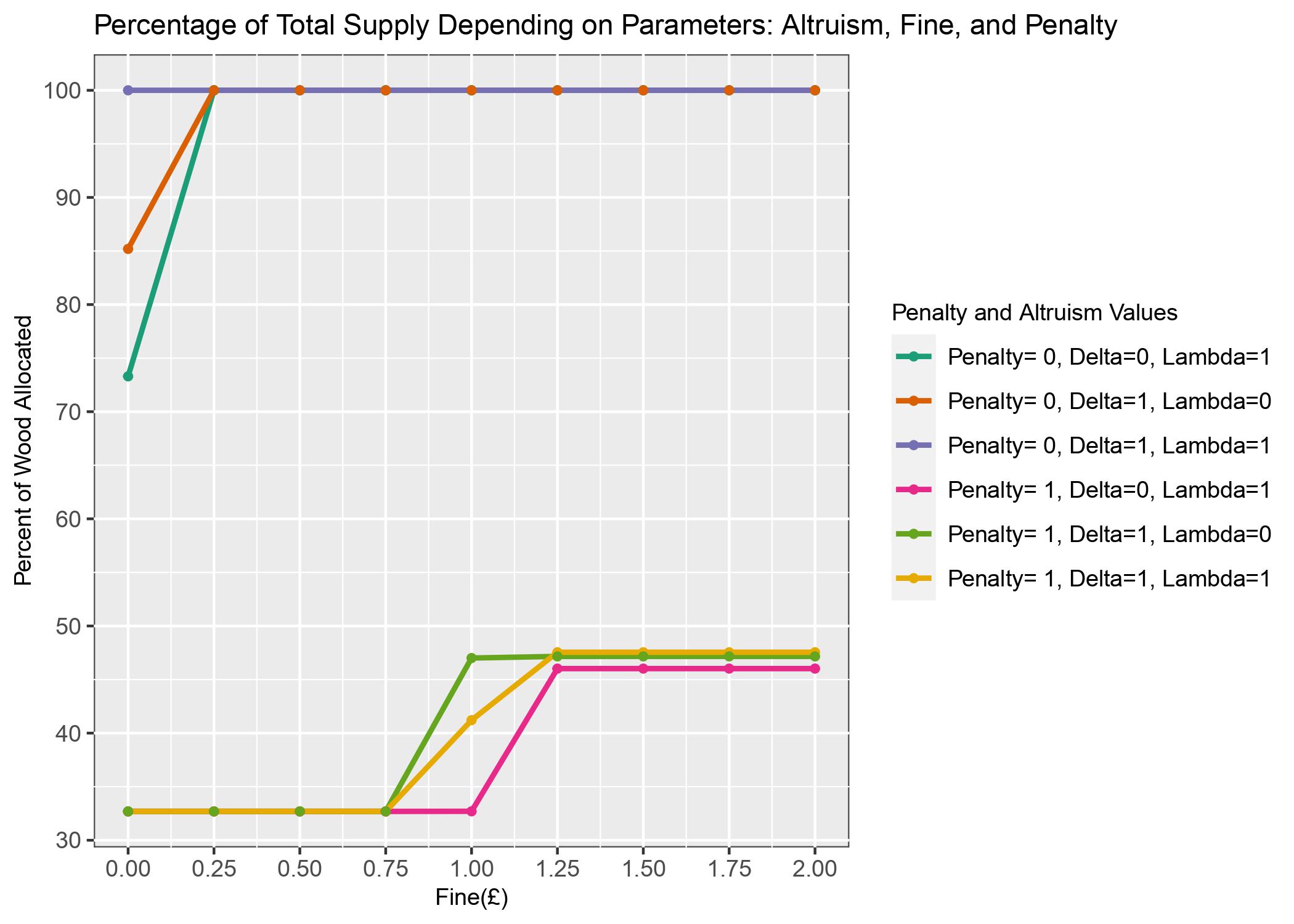
Figure 2: The effects of altruism, fine and penalty on \(\overline x\) as a portion of total supply

5.2.2 Villagers Behaviour to Harvest Legally or Illegally

Altruism has no effect on the decision-making of villagers when penalty=0, i.e. all wood supply is allocated. Although there is illegal activity at \(\phi\)= 0 it is irrelevant because neither villages or community leaders incur a loss. It is clear that fine does have an effect, illegal behaviour generally peaks when there are no repercussions, but once \(\phi\)> 0 all illegal harvesting subsided (seen in figure 3). In all cases the villages acquired all wood allocated to them before harvesting additional illegal wood.

Table 1: Harvest behaviour of Villages when penalty= 1

	Village 1	Village 2	Village 3	Village 4
Illegal Harvesting Ends (y=0)	\(\phi\) = 1, except for \(\delta\)= 1, \(\lambda\)= 1 which ends at \(\phi\) = 1.25	\(\phi\) = 1 for all altruism combinations	\(\phi\) = 1.25, except for 0 which ends at \(\phi\)= 1	\(\phi\) = 1.25 for all altruism combinations
\(\delta\) = 0, \(\lambda\) = 1	Peak quantity harvested (9.09) at = 0.25, very little harvested illegally after \(\phi\) > 0.25 \(\phi\) = 0.5, y= 0.7 \(\phi\) = 0.75, y= 0.3	\(\phi\) = 0 total harvest= 4.62, \(\phi\) = 0.25 total harvest= 5.27, \(\phi\) > 0.25 total harvest= 9.75 and village 2 will cut illegally or legally to acquire it	\(\phi\) = 0, y= 32.85 all harvest is illegal \(\phi\) = 0.25 y= 3.6 \(\phi\) = 0.5, y= 0.9 \(\phi\) = 0.75, 0.4	\(\phi\) = 0, y= 3.35 \(\phi\) = 0.25 y= 4.39 \(\phi\) = 0.5, y= 0.86 \(\phi\) = 0.75, 0.4 \(\phi\) = 1, y= 0.08 slightly increasing total harvest to the same amount allocated for \(\phi\) > 1
\(\delta\) = 1, \(\lambda\) = 0	\(\phi\) = 0, y= 3.14 \(\phi\) = 0.25 y= 3.13 \(\phi\) = 0.5, y= 1.33 \(\phi\) = 0.75, 0.64	\(\phi\) ≤ 0.5 total harvest= 13, \(\phi\) > 0.25 total harvest= 9.75 and village 2 will cut illegally or legally to acquire it	\(\phi\) ≤ 0.25 total harvest = 23.3 \(\phi\) = 0.5, y= 1.4 \(\phi\) = 0.75, y= 0.71	\(\phi\) = 0, y= 3.35 \(\phi\) = 0.25 y= 2.59 \(\phi\) = 0.5, y= 1.18 \(\phi\) = 0.75, 0.6 \(\phi\) = 1, y= 0.08 slightly increasing total harvest to the same amount allocated for > 1
\(\delta\) = 1, \(\lambda\) = 1	Total harvest slowly decreases as fine increase, the difference between highest and lowest harvest is 1.47 units	\(\phi\) ≤ 0.25 total harvest= 5.17, \(\phi\) > 0.25 total harvest= 9.75 and village 2 will cut illegally or legally to acquire it	\(\phi\) ≤ 0.25 village 3 harvests 64% of total supply (33.23 units) \(\phi\) = 0.5, y = 1.8 \(\phi\) = 0.75, y= 0.9	\(\phi\) ≤ 0.25 y= 2.01 \(\phi\) = 0.5, y= 1.51 \(\phi\) = 0.75, 0.75 \(\phi\) = 1, y= 0.33 slightly increasing total harvest to the same amount allocated for > 1

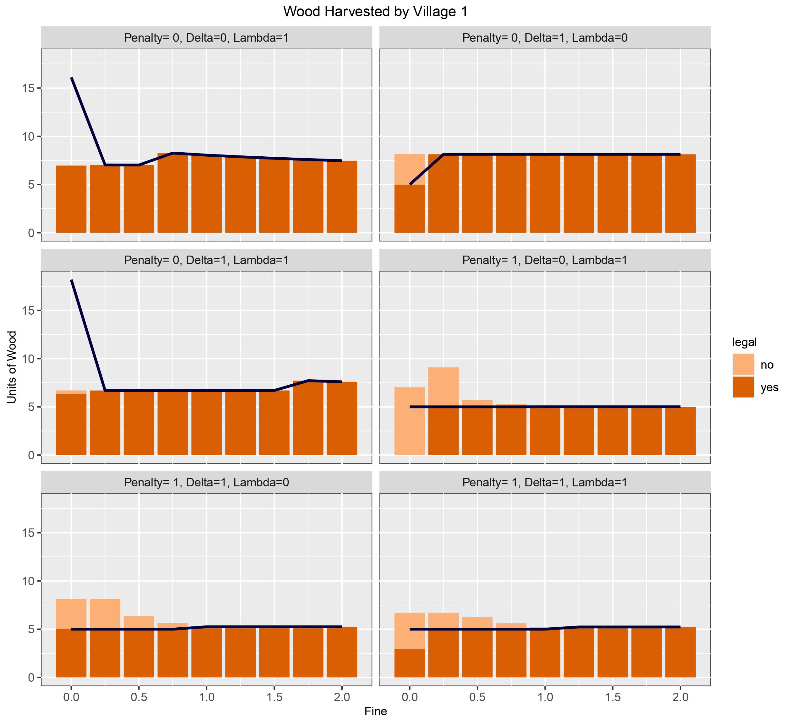
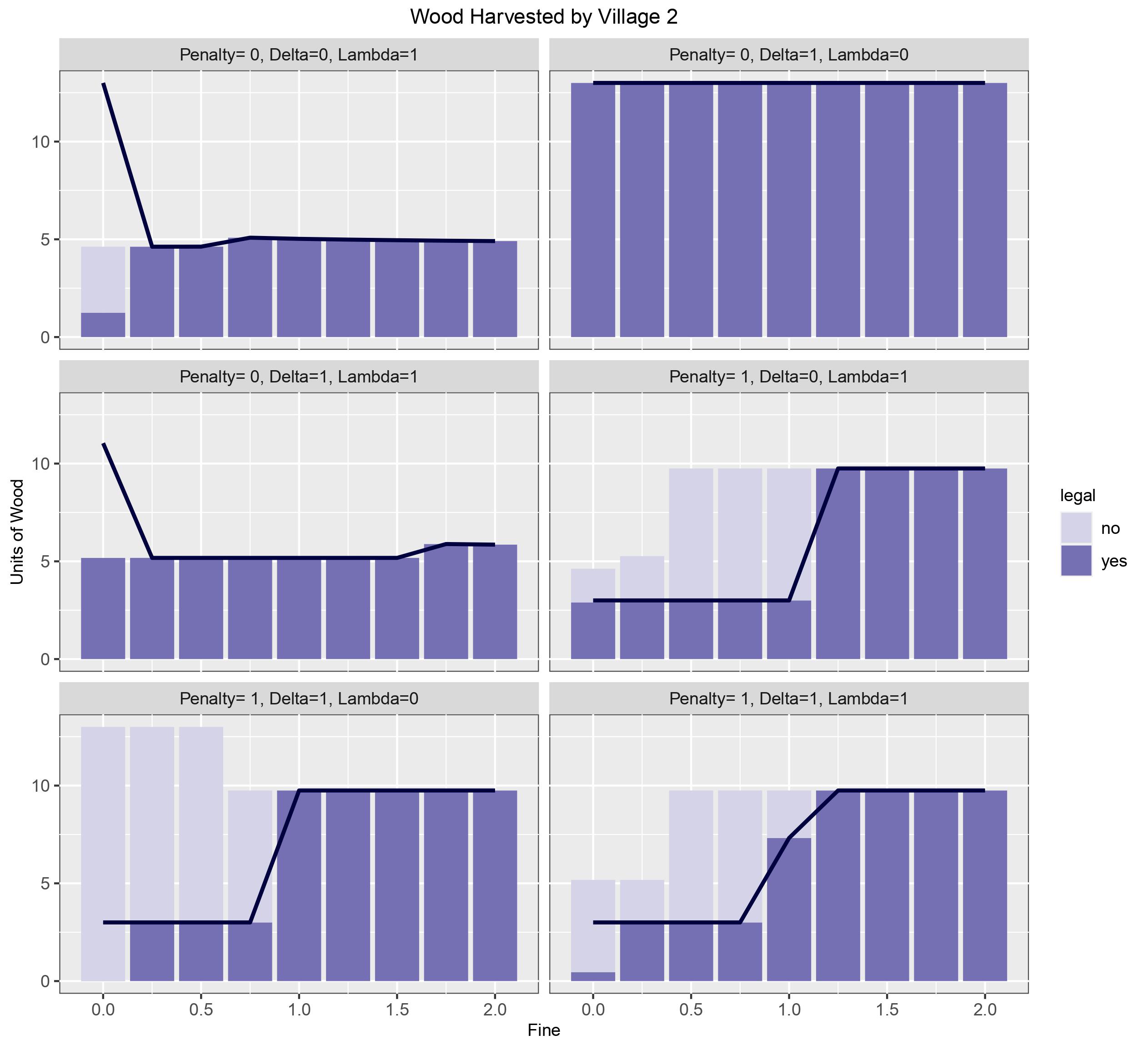
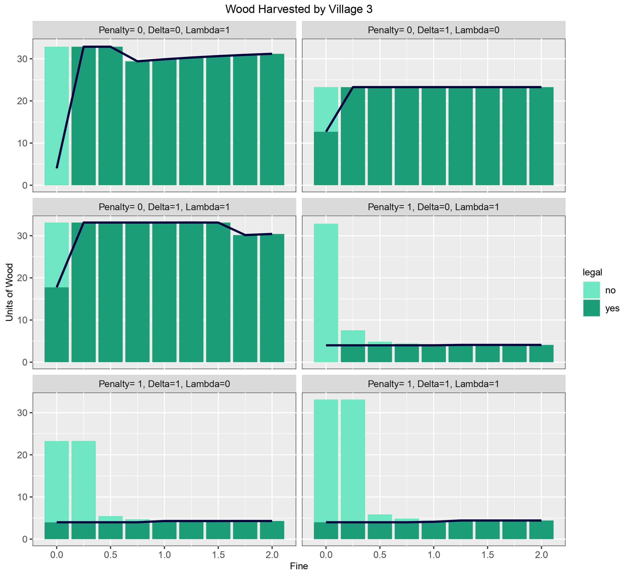
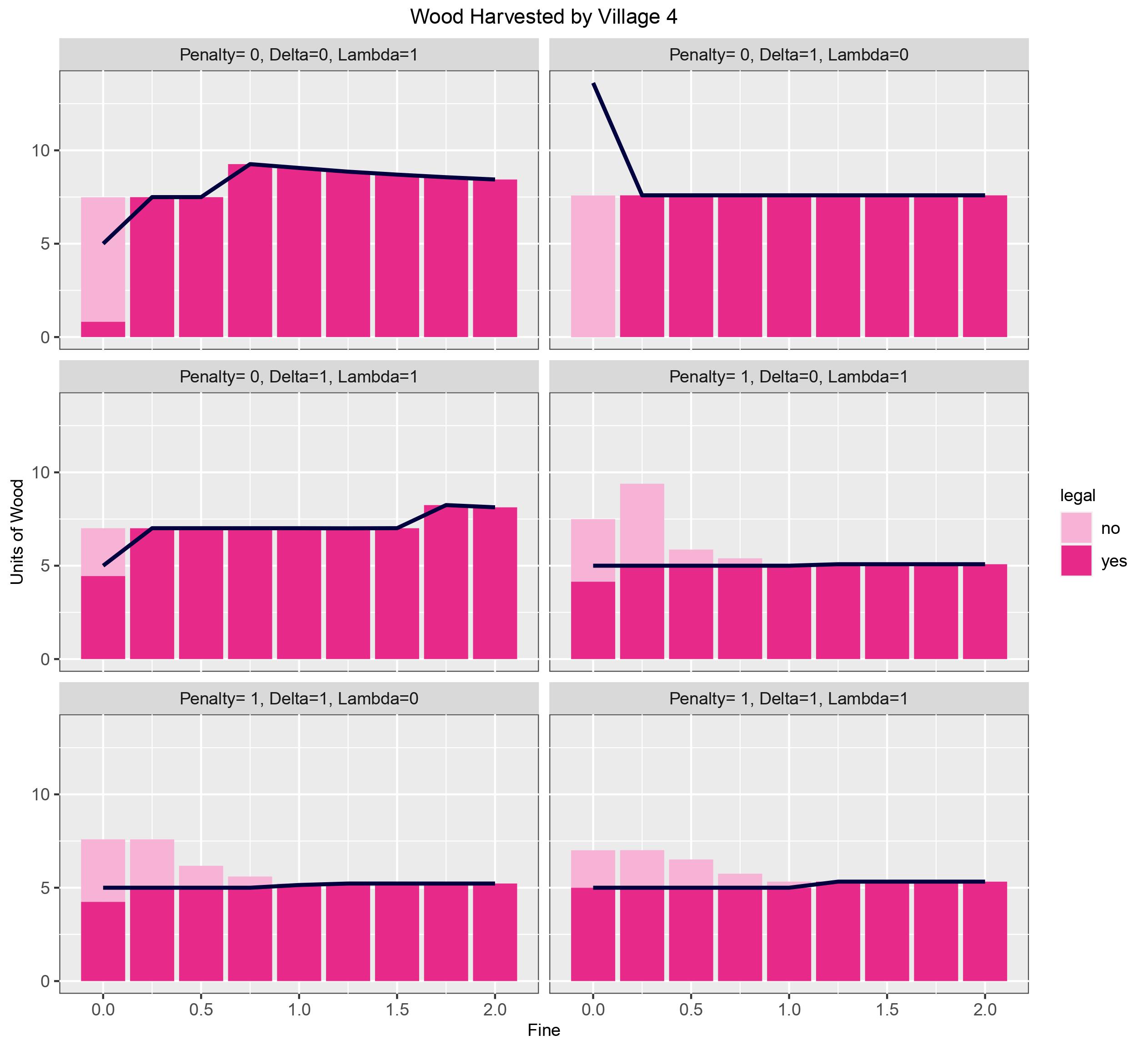
Figure 3: Quantity of wood harvest legally and illegally by all villages. The darker shades represent legal wood cut, and the dark blue line indicates how much wood was allocated to the village based on fine and altruism

5.2.3 Welfare

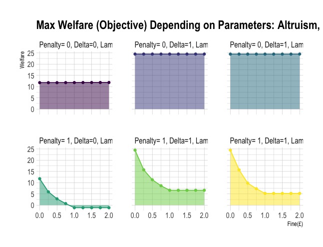
Figure 4: Welfare for the Upper Level is a summation of the welfare for all 4 villages less penalties. The top row has outcomes for penalty= 0, and the bottom row for penalty=1.

Although the top middle and right graph look the same they differ by approximately 2 decimal place. As fine increases, welfare for both graphs fluctuate around the 4th and 5th decimal place. In both cases welfare= ~24.5. The top right graph's welfare= ~11.8 (also with minor fluctuations as fine changes), it is much lower than the other two in its row because \(\delta\) =0, that aspect of the altruism score carries the majority of the weight in the score and it is now excluded.

For penalty= 1, the objective somewhat plateaus when fine ≥ 1, because there is little illegal harvesting, and the penalty for the leader allocating more than minimum demand is stagnant. For fine < 1 it was beneficial for the upper level to allocate less with the expectation of illegal harvesting. Welfare dramatically decreased as fine increased. Individual villages' welfares are penalise but overall it was less harmful than if the leader took the loss.

5.3 High Point Relaxation- Fixed \(\overline x\)

Setting penalty=fine=1 (the value at which there is the most volatility for upper level decisionmakers), and \(\delta\) = 1, \(\lambda\) = 1 (the values at which all villages care about themselves and the environment, unless spiteful) high point relaxation is used to find \(\overline x\). The values for \(\overline x\) are in Table 2 below.

Table 2. Values for \(\overline x\)

	Village 1	Village 2	Village 3	Village 4
Demand	5	3	4	5
Woodlot 1	0	3	0	6.4772
Woodlot 2	5	0	4.28746	0

5.3.1 Villagers Behaviour to Harvest Legally or Illegally

Village 1

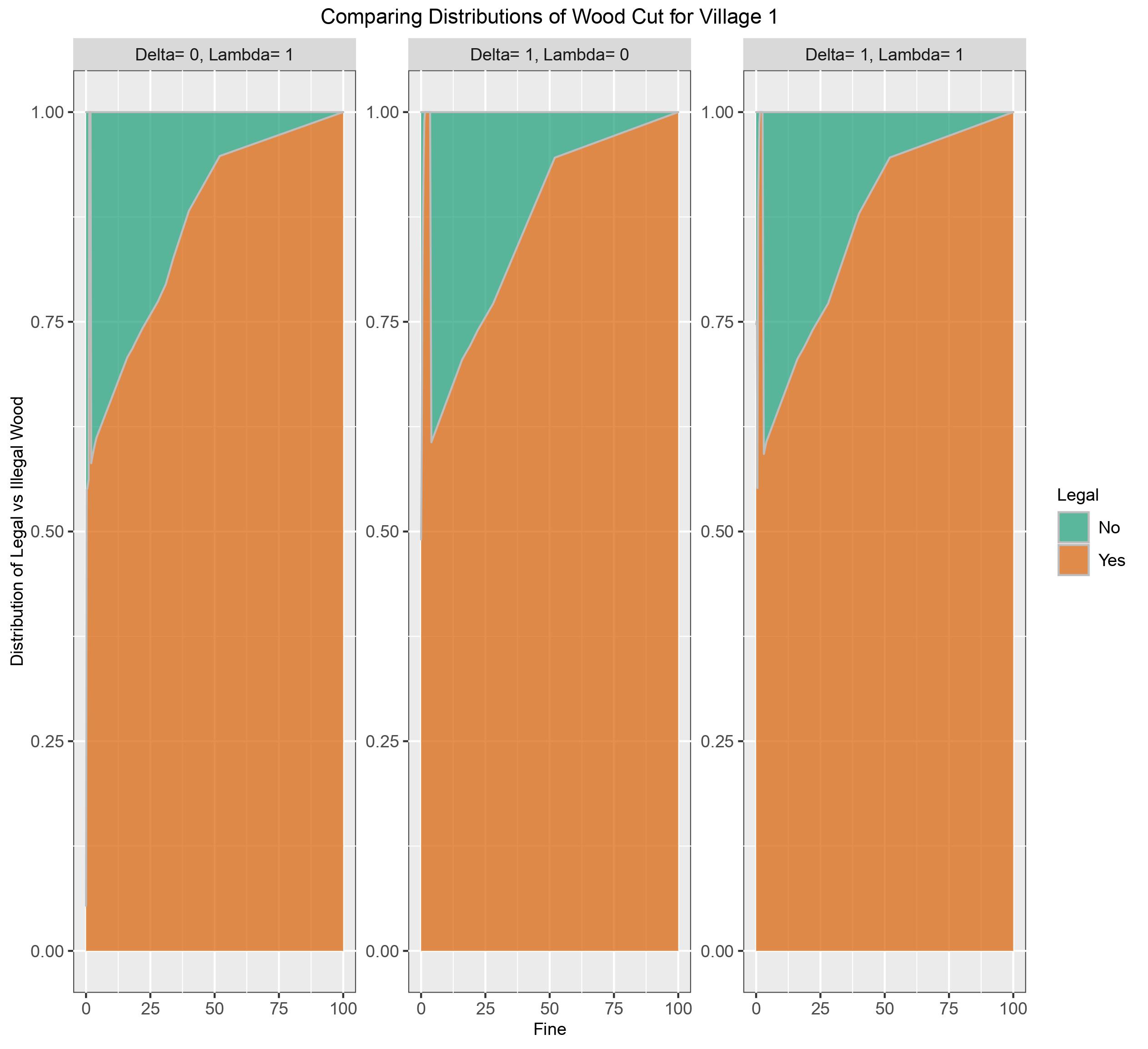
Figure 5: Distribution of legal and illegal wood cut by Village 1 for the different combinations of altruism as fine ranges [0,100]

Village 1's peak illegal behaviour occurs at fine= 0.25 for all combinations of altruism, and is highest when \(\delta\) = 0, \(\lambda\) = 1 at 45%. Village 1 was allocated 5 units of wood, the equivalent of its minimum demand. There is a period when 1.25 < fine < 3, (4,2) (left to right, depending on altruism) where village 1 does not cut any illegal wood, after this it picks back up. Village 1's preference towards illegally cutting wood slowly wanes as the fine is increased, eventually ending at fine= 62 (or 63 when \(\delta\) =0, \(\lambda\) = 1).

Village 2

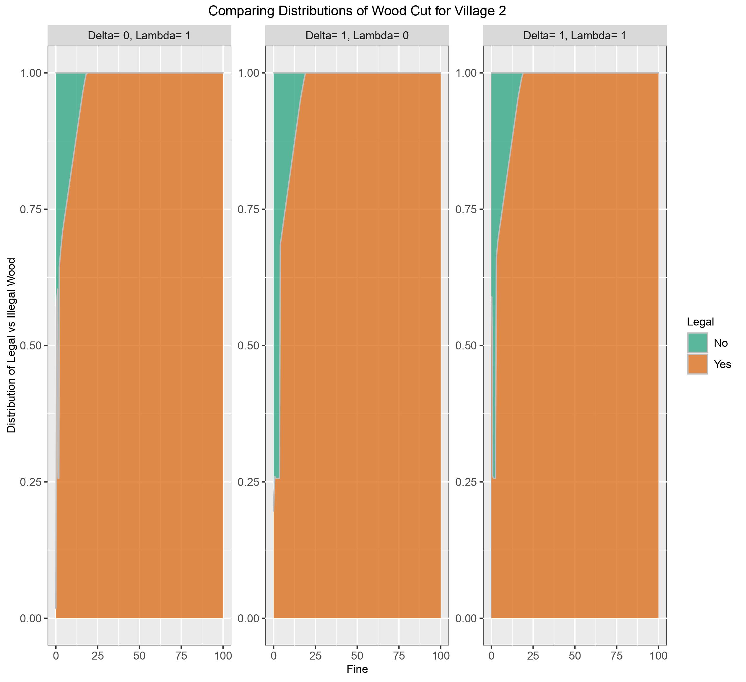
Figure 6: Distribution of legal and illegal wood cut by Village 2 for the different combinations of altruism as fine ranges [0,100]

Village 2 was allocated its minimum demand, 3 units of wood. The shortest range of high illegal behaviour occurred in the right graph where it peaked at 74% for 1.25 ≤ fine ≤ 1.75, dropping to 33%, prior to fine= 1.25% illegal harvesting averaged 41% of total harvest. The left graph peaks at 74% illegal harvesting when the fine ranges between 0.75 and 2. Before the peak the average illegal harvest was 42% and afterwards it drops to 34%. In the middle graph village 2 illegally harvests 74 to 76% for 0.25 ≤ fine < 3.5, falling to 31% and continuing to quickly fall. In all 3 cases of altruism, when fine ≥ 19 village 2 quits all illegal behaviour. At its peak harvest village 2 harvested approximately 4 times more than what was allocated to it. The behaviour is consistent through all combinations of altruism parameters although the fine ranges vary for peak illegal harvesting.

Village 3

Figure 7: Distribution of legal and illegal wood cut by Village 3 for the different combinations of altruism as fine ranges [0,100]

Village 3' behaviour is different from all others as it harvests illegally at the highest fines even though it did not when the fine was lower. When \(\delta\) =1, \(\lambda\) = 0 village 3's harvest behaviour is unlike all others when ≥ 1, its illegal harvesting fluctuates - 87%, 14%, 94% and 18% for = 0.25, 0.5, 0.75, 1 respectively.

Table 3. a description of Village 3's illegal harvesting behaviour for each altruism combination at different values for fine (\(\phi\) )

Behaviour	\(\delta\) =0, \(\lambda\) = 1	\(\delta\) =1, \(\lambda\) = 0	\(\delta\) =1, \(\lambda\) = 1
Peak illegal harvest percent, and value of fine	43%, \(\phi\) = 0.25	97%, \(\phi\) =0.75	87%, \(\phi\) =0.25
Values of fine when illegal activity quickly decreases to 0	0.25 < \(\phi\) < 1.25	N/A	0.25 < \(\phi\) < 1.25
No illegal harvesting	1.25 ≤ \(\phi\) ≤ 1.75	1.25 ≤ \(\phi\) ≤ 0.35	1.25 ≤ \(\phi\) ≤ 2.5
Change in behaviour- begins to harvest illegally again, and there's a slower rate of change. including local peak illegal distribution	36%, 1.75 < \(\phi\) < 32	32%, 3.5 < \(\phi\) < 32	34%, 2.5 < \(\phi\) < 32
No illegal harvesting	32 ≤ \(\phi\) ≤ 53	32 ≤ \(\phi\) ≤ 53	32 ≤ \(\phi\) ≤ 52
Illegal behaviour slowly climbs again, illegal share at fine=100	3%, 53 < \(\phi\) ≤ 100	3%, 53 < \(\phi\) ≤ 100	3%, 52 < \(\phi\) ≤ 100

Village 4

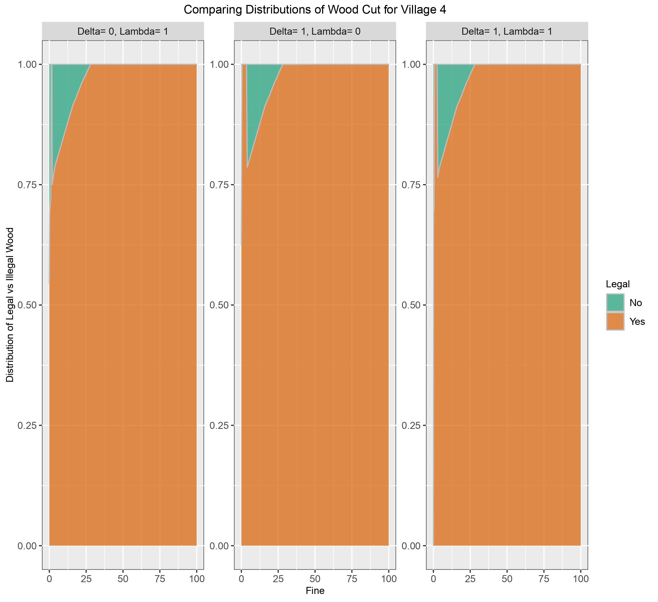
Figure 8: Distribution of legal and illegal wood cut by Village 4 for the different combinations of altruism as fine ranges [0,100]

For all combinations of altruism, village 4 halts illegal harvesting at \(\phi\) = 29. As seen in the graphs there is also a range of fine values at which the villages do not harvest illegally; they are 1.25 < \(\phi\) < 2 (\(\delta\) = 0, \(\lambda\) = 1), 0.5 < \(\phi\) < 4 (\(\delta\) = 1, \(\lambda\) = 0), and 0.5 < \(\phi\) < 3 (\(\delta\) = 0, \(\lambda\) = 1). Before pausing illegal activity for the fine values mentioned village 4 is most likely to harvest illegally. In the second peak after the pause, total harvests consists of 21% to 25% of illegal wood.

5.3.2 Welfare

As fine increases, so do the costs to acquire each unit of wood beyond minimum demand, and so even though illegal harvesting decreases with the increase of fine, overall welfare decreases. For all three combinations of altruism, minimum welfare= ~ -48 to -50 occurs at fine= 16. All villages are illegally harvesting at this time, with the average percentage of their harvest being done illegally at 14.6% with standard deviation= 9.9%. Villages 1, 2 and 4's illegal harvesting gradually lessens after this. Welfare is lowest when \(\delta\) = 0 (green line), compared to \(\delta\) > 0. Ultimately, negative welfare means villages are not happy about the overall outcome nor or they financially compensated, and are taking a loss by taking part in the community based system.

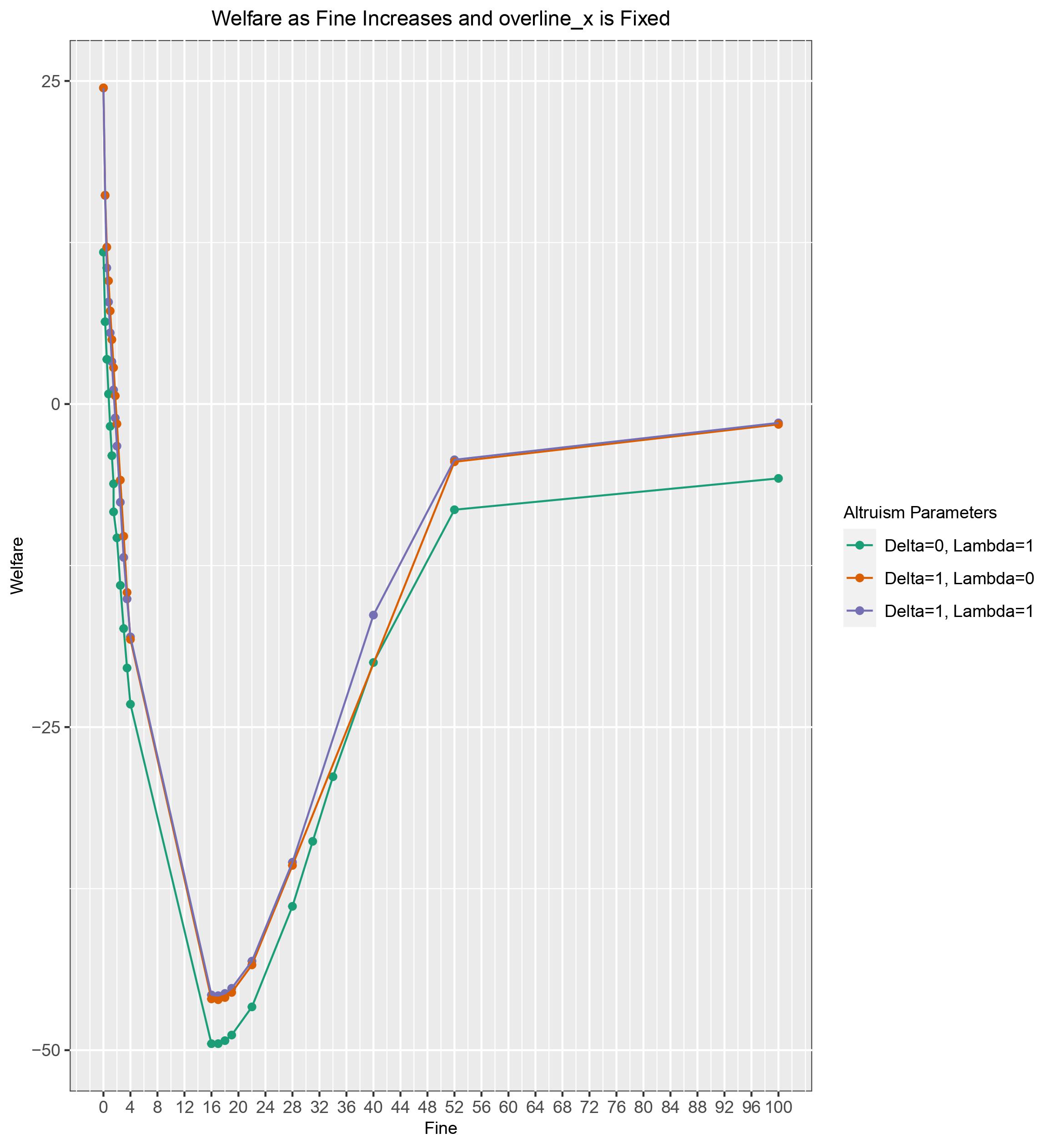
Figure 9: Total Welfare as fine increases for each combination of altruism.

6. Discussion

Because all data used in the experiment is random there are no definitive results or outcomes from these tests, only a better understanding of if the model can aide in the allocation of wood for rural Malawians. Using bilevel optimisation and KKT reformulation allowed us to observe the decisions of both committee and villages as they simultaneously reacted to parameters. While high point relaxation focuses on the committee's objective and is used to implement the committee's allocation of wood as an unchanging parameter in the bilevel model to provide insight into the villages' behaviour post wood allocation. The model, as is, did not emulate the expected behaviours of the villagers or committee well, and maximising welfare created an unrealistic controlled environment.

The community leaders' intention of impeding illegal harvesting was successful when the entire supply was allocated (penalty= 0) , all villages received higher than their demands and there was a fine present. Penalising the community leaders produced a tradeoff effect with fine; maximising welfare meant that one of the two parties would have to absorb the costs for harvesting beyond the demand minimum. If fine < penalty the community leaders allocated less increasing the likelihood that villages would illegally harvest thereby becoming accountable for the fine. If fine > penalty the community leaders allocated more to villages because they know meeting minimum demand is not sufficient for villages to make any profit and it costs the objective function less if the community leaders paid the penalty. Although more wood is allocated, the committee never allocates in excess of 47.5% of supply meaning that penalising the leaders is useful for barring total supply from being allocated. Since the penalty's influence is not stand-alone it does not matter what the value of the constant is, what matters is its relation to fine.

Evidently, penalising the leaders was not the best approach to avoiding the allocation of all wood. The simultaneous decision-making of the model for all decision variables is a property of bilevel optimisation, and so the trade-off effect is unavoidable with both fine and penalty present. To eliminate this effect, one of the parameters must be removed. Fine is instrumental to the allocation problem, and so if bilevel optimisation is to be used the quantity of supply used in the model should all be permitted for allocation without penalty.

Parameters delta and lambda in the altruism portion of the objective function had little effect on the community leaders. Their influence was visible when fine = penalty \(\pm\)0.25 and penalty > 0. For \(\delta\) = 1, \(\lambda\) = 0 the utility of each village is impacted by the outcome of others less, therefore their utility is higher when they focus more on themselves. In this case, the community leaders increase wood allocation at fine= 0.75, because fine < penalty selfish villages are more likely to take financial risks earlier on. When \(\delta\) = 0, \(\lambda\) = 1 villages are more altruistic because they care both about others and others' opinions therefore community leaders are less concerned about illegal harvesting and can risk increasing supply later on at fine= 1. Lastly, when \(\delta\) = 1, \(\lambda\) = 1 the utility for all villages are highest when they themselves and all other villages prosper. Whereas the previous two jumped from total allocation= 24.72% to 47.54% in one fine increment (0.25) this one increases gradually over two increments. As there is no polarised preference in the altruism score portion there is less pressure on the community leaders in comparison to when one of the parameters is 0. Each village's \(\alpha_i\) value gives the community leaders insight into the villages' harvesting behaviour and their outlook on others and the environment. Villages 1, 3, and 4 all have \(\alpha_i\) > 0 (are altruistic) and were allocated minimum demand by the community leaders. Whereas, village 2's \(\alpha_i\) < 0 indicates spitefulness, and are therefore more likely to harvest illegally; the community leaders allocated village 2 3.25 times their minimum demand. Village 2's spitefulness means that its utility does not benefit when others prosper, it actually suffers, and to counteract that village 2 needs to harvest more to potentially receive a positive altruism score, and this is why the community leaders allocate more to village 2, to offset that.

The aforementioned trade-off effect between penalty and fine also altered the villages' behaviours. When there was no penalty, and all wood was allocated the villages did not harvest illegally, and they all harvested their max legal units of wood. When penalty= 0 and fine= 0, depending on how much was allocated to them they may choose to harvest all or some, and some chose to harvest illegally. Although the behaviours of villages' with these two constants are irrelevant because their behaviours are not curbed in any way.

With the exception of village 2 all villages harvest the max amount allocated to them by the committee leaders when penalty= 1 and fine ≤ penalty, and then harvest the remainder illegally, continuously decreasing the illegal amount as fine increases. For village 2, as fine increased they harvested more illegally until committee leaders increased their allocation. When almost all the importance is placed on village 2 (\(\delta\) = 1, \(\lambda\) = 0) it cares most about increasing its utility by harvesting more when the fine is lower, grabbing the second largest share of total supply, because its utility does not benefit from the boost of \(\lambda\) > 1. In the other 2 cases where \(\lambda\)= 1, village 2 benefits when the other villages harvest more therefore it does not need to harvest as much early on. But as fine increases the other villages harvest less and village 2 chooses to increase its utility by increasing its amount of harvested wood even though it comes at a penalty.

Shifting \(\overline x\) from a variable into a parameter allowed us to better focus on the decision-making of villages. We thought this was pertinent to our research as it is unlikely that committee leaders would adjust their allocation to alleviate the cost burden from villages. To obtain \(\overline x\)'s values the model was run using high point relaxation with penalty=fine. As we know, penalty=fine produces the most variability in allocation because both parties are penalised equally and so neither is given favourability. The results were villages 1 and 2 were allocated minimum demand, 5 and 3 units of wood respectfully; and villages 3 and 4 were respectfully allocated 1.07 and 1.3 times their demand.

For all villages with \(\alpha_i\) > 0 there is a range of lower fine values where they choose not to illegally harvest, usually around 1.25 to 2 (and sometimes up to fine=4). The range in which villages are more cautious to not harvest illegally is widest when \(\delta\) = 1, \(\lambda\) = 0, that is when their utility is greatly affected by their own behaviour and not so much by others. Conversely it is most narrow when \(\delta\) = 0, \(\lambda\) = 1 and their own behaviour has less influence on their utility, so they're willing to take more risks. Once the fine threshold is where there is no illegal harvesting is overcome the villages all begin to harvest illegally again, steadily lessening as the impact of the fine is too great and they quit harvesting illegally (figures 5, 7, 8). Village 3 uniquely harvests illegal at fine ≥ 53, although it never surpassed 1 unit of wood, the quantity of wood kept creeping up higher and higher as with the fine (figure 8).

For villages with \(\alpha_i\) < 0 , the opposite occurred, during those fine values in which the others did not harvest illegally, village 2's peak illegal harvesting behaviour occurred. Then descended to 0 illegal harvest much quicker than the others at fine= 19. It is difficult to make an absolute observation for villages with \(\alpha_i\) < 0 because there is only one village in this category and its behaviour is likely to be influenced by other parameters.

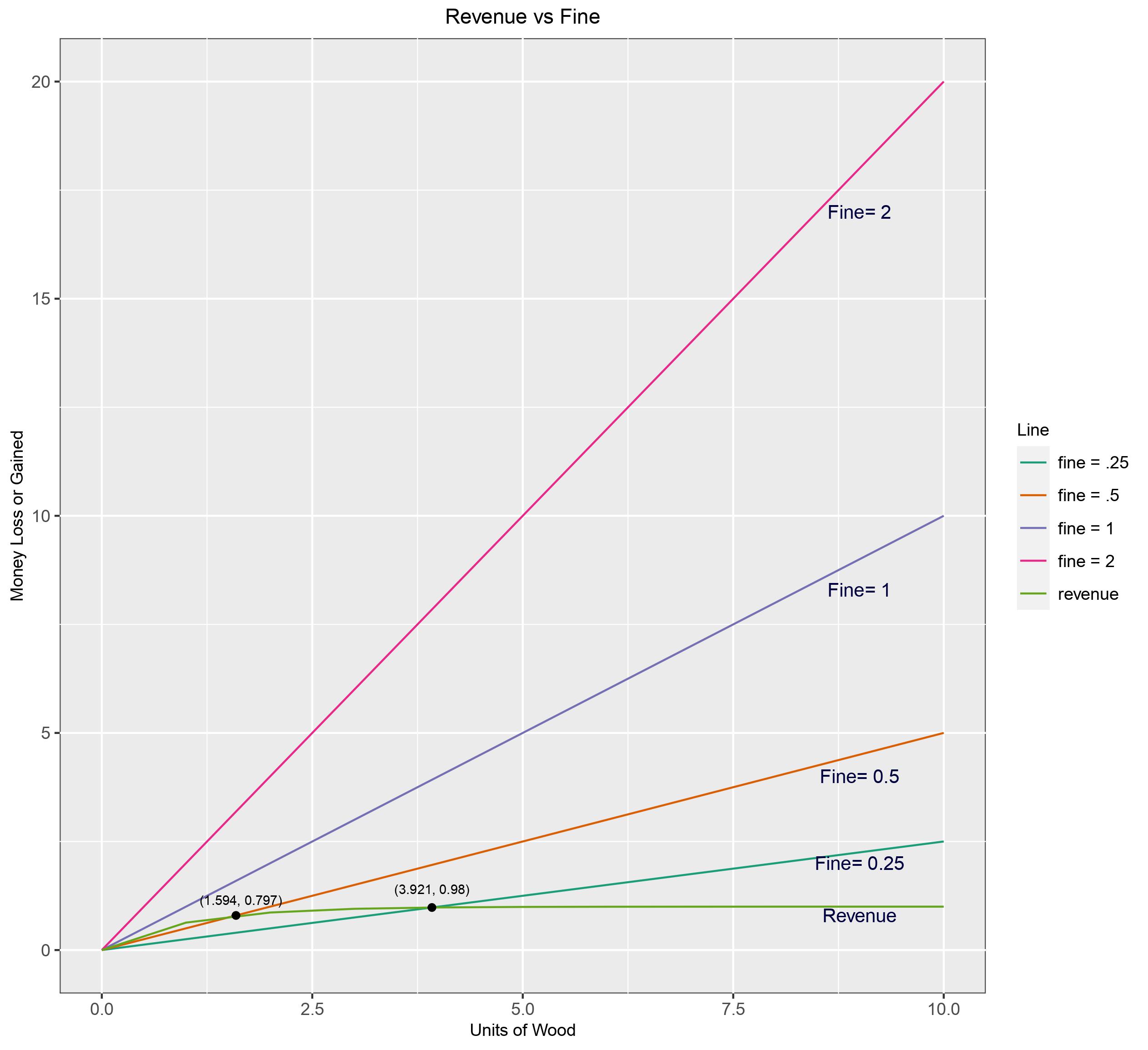
Figure 10: The relationship between revenue at selling price per unit = 1 and fine = 0.25, 0.5, 1, and 2

Revenue earned from selling each unit of wood for 1 is displayed in figure 10. The concavity in the line indicates that the utility payoff decreases with each additional unit of wood, and the greatest utility payoff at per unit value occurs at x+y-d= 1 (revenue= 0.63). Fine on the other hand increase linearly. From the graph we can see that when fine = 0.25 revenue and fine intersect at (3.921, 0.98) and fine= 0.5 intersects at (1.594, 0.797), fine=1, 2 do not intersect with revenue. Therefore when fine= 0.25 a village neither gains or loses anything if they illegally harvest up to 3.921 units of wood, and as the fine increases the quantity of wood that can be harvested without penalty quickly decreases.

It seems as though constants Income and Fee may have had an inverse effect on the decisionmaking of villages. For example village 3's balance of income-fee is greater than all others, but was the village likely to harvest illegally later on. Villages with a higher balance are expected to depend less on wood for income, and would therefore be less likely to harvest, but it seems as though because it’s balance was already most positive it was the village who could take the most financial risk. The outcomes do not suggest that Wood Per Trip (WPT) played a large role in dictating how much wood villages collected. Village 4 can carry 8 units of wood, but even when there was no fine for illegal harvesting they did not harvest more than 7.6 units of wood. The preference between woodlots depending on distance will be later dissected when reviewing the model itself.

Welfare comprises of two main components financial profit or loss and an altruism score, which does not help us understand how well or poorly villages are doing financially. Figure 11 (below) displays the average financial balance of the villages versus the average altruism score as fine increases. We can see that while altruism remains positive their average financial balance falls to -13.183 and constantly remains negative after fine= 0.5. Ultimately, if the villages cannot afford to live regardless of how well the environment or their neighbouring villages are doing they will never be happy.

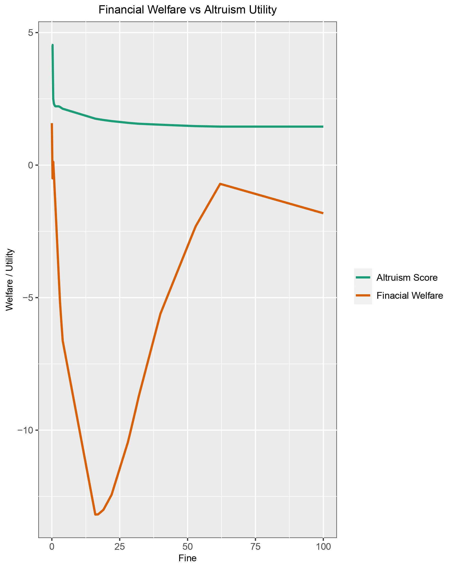
Figure 11: Comparing average financial balance to average altruism amongst villages as fine increases

6.1 Data Limitations

Data used in this case study was pseudo randomly created in AMPL, and therefore does not mimic real data. Using a single demand unit for each village did not provide enough insight into their needs or their dependence on wood. We understood that villages that harvest wood sometimes do so to meet their own demands, and in other instances for economic income to support their families. Without having the real data we were not able to decipher between the different types of demand. Furthermore villages located near to urban cities are more likely to sell wood products, so their needs for wood are dictated by those of their customers. The data needed to be expanded to create some variation or a probabilistic element to calculate the chance of needing more of less wood for each village. Additionally, those villages are subject to elastic demand, and the prices they sell units of wood for may change at any time. Data assigned to each village was done uniformly through a set minimum and maximum, because of this a village that received a low income also receive low demand, and a village that received higher income was also assigned higher demand. Chilongo (2014) and the World Bank (2020) explained that villages with lower incomes will have higher demands because they depend on forest products more. This relation between demand and income was not reflected in the data used and is likely to have affected the outcome.

Villages must pay a fee to be a part of the scheme. For many it is too expensive and so they choose to risk harvesting illegally. Regardless of if a village takes part in the community based system or not they all harvest from the same forest reserves, and therefore there is a chance that the supply allocated to a village within the system may have been previously harvested. The fees villages pay are dependent on the units and types of trees they demand. Our data was not segmented based on tree type and fee was not relative. We were not privy to details about tree supply density or village preferences for trees. To create competition amongst the villages so they can arrive at a Nash equilibrium we used k=N/2, but it is unknown to us how supply is segmented or accounted for.

We suspected that the distance of legal wood may impact illegal harvesting. Knowing that villages in the case study are within 5 kilometre from the forest reserves, we used that figure as an upper bound on the assigned distance from villages to forest data. This decision may have been shortsighted as the committee may not necessarily use the forested areas closest to the villages for allocation. The upper limit on maximum travel was meant to play a role in the decision making of the villages, but the distances between village and forest were all too similar and short. Not assigning any longer distances did not allow us to observe if a village was not pleased with the distance of legal wood allocated to them, or if they may have chosen to harvest illegally instead because the cost to travel for illegal wood was cheaper and worth the risk. Some of these data limitations were meant to be avoided by using GIS techniques to acquire the data, but due to time constraints they were not acquired.

6.2 Model Limitations

Beginning with the objective functions' sub-equation h₁- concavity is a requirement of utility functions; that guided us to formulate h₁ using \(1- \epsilon^{-\beta ( \sum_j(x_{ij}+y_{ij}-d_i))}\). In retrospect this may not have been the best method for achieving concavity as it created many limitations. Its main purpose was to understand how each villages utility increase as quantity of wood harvested increases. This calculation needed to include how much was earned from selling excess wood and how much was loss to paying fines for illegal harvesting and several other constants. Because of the initial sensitivity of exponential and its insensitivity to larger numbers we were limited to using \(\beta\) < 1. When using a much larger selling price (\(\beta\)), revenue was already much too large for one unit of wood to provide the sensitivity needed from the h₁ sub-equation. It also placed restrictions on the fine which is why it had to be placed outside of h₁. When fine was included in h₁ it created a flaw to the model where even though villages did not harvest up to their legal amount (\(\overline x = x\)) they were harvesting illegally from the same area, because when scaled using the exponential the difference between 2 or 3 units of wood harvested illegally instead of legally became insignificant.

Villages are limited by the capacity of wood they can carry on each journey. The h₂ sub-equation used for calculating travel cost did not round up the quantity of wood carried. This affected the overall out come in two ways: 1) travel costs were calculated incorrectly and were all cheaper than they should be and 2) the max travel constraint which uses the same equation without cost of fuel per kilometre calculated the distance traveled in proportion to how much wood was collected.

The original altruism and spitefulness utility function by Levine (1998) was meant to be used one-on-one, our adaption averaged the utility loss or gained by villages i' and also gave the opportunity to remove or place less importance on the utility gained from the harvest of village i. The altruism score is heavily skewed by village i's gain, and in our opinion that encouraged village i to be behaviour more selfishly. Using = 0 we removed that portion of the altruism score, and were proven incorrect. From figures five through eight villages were more greedy when fines were lower and \(\delta\) = 0. By using \(\lambda\) rather than \(\lambda_i\) we grouped the outlook of villages on others. It would have been beneficial to use \(\lambda_i\) to see how the interactions behaviours may have changed based on how each village felt towards another specifically. In a real situation all villages would not have the same opinions all at the same time.

Harvesting is performed cyclically, but the model was built for a one time use. Conserving and rebuilding the forests are acts that may take many decades, so it is crucial to understand the harvesting habits of the villages and how their needs change over time. The model did not have any components for this nor did we have access to this information. One of the most harmful limitations of the model is that supply needs to be greater than demand, rendering the model useless if there was a shortage. In order to aid in forest conservation the committee may sometimes limit the supply intended for that round of harvest regardless of demand. If the model cannot perform in this event then it is not that helpful to the committee.

6.3 Recommendations

Computationally, the model is constrained to values of N ≤ 10. The simplest path to increase the value of N is using a computer with greater CPU and memory, which will also eventually be limited at some other greater value of N. Another option is for the committee to use a best response dynamics heuristic. The committee can first solve a relaxed version of the bilevel model, solving only for the committee's best case scenario using High Point Relaxation (HPR). As a starting point we can substitute the decision variable values from HPR into the bilevel model. Selecting a single village we fix the decision variables of all other villages, and optimise for the selected village. The new values of legal and illegal wood for the selected village are updated and become fixed. A second village is then selected and the same process is performed until all villages have been selected and no village has a strictly better solution than the current one. With this method each village chooses what is best for them at that time given what the others are doing seeking a pure Nash equilibrium (Roughgarden, 2013). If each village can continue to improve their outcome then an equilibrium is unachievable.

Another approach to finding estimated optimal solutions when branch-and-bound is infeasible is using heuristic search algorithms. Heuristic search algorithms are computationally cheaper to carry out in comparison to branch-and-bound, and the longer the system is left search the better the solution. Though this approach is only recommended when the value of N is large as heuristic search algorithms are not easy to formulate.

Ultimately, altruism cannot feed a family. A profit does, and combining altruism with financial welfare did not benefit the villages financially. The two sub-sections in the objective functions can be considered conflicting. On one hand villages want to prosper financially, and on the other they want to save the environment, but with their current habits they cannot do both. Altruism and financial welfare should not have been initially grouped into one function. Each programming model should have been made bi-objective and then using compromise programming formulation they could have been combined. The compromise programming approach was suggested by Zeleny (1982); it would allow the committee to find compromises amongst conflicting criteria. The merged objective function contains an 'ideal solution' or 'utopia point' F^*_N that will simultaneously optimise all of the original F_N functions where N= 1,...,n. An 'ideal solution' is obtained by optimising each F_N independently within a bounded set of alternatives, i.e. it is a compilation of all the singular objective functions. However, it is rare to have a single solution because there are usually trade-offs or compromises amongst the objectives. The merged objective function's goal is to minimise the distance of from the boundary of feasible solutions to the ideal solution (Chattopadhyay, 2001, Ringuest, 1992).

One of the limitations of using KKT reformulation for bilevel problems is that lower level problem cannot host binary variables. Yeu and You (2017) propose using optimal value reformulation and a decomposition algorithm which is capable of solving bilevel problems with binary variables in the lower level. As is, our model does not include villages who are not taking part in the community based system. It would be helpful if they could be included in the model so the committee can include their potential behaviour. A binary variable representing villages in the scheme or not in the scheme can be used in the lower level problems. Optimal value reformulation fixes the lower level problems' binary variables transforming it into a continuous convex model. Once in this form KKT conditions can be used to reformulate the followers' problems. Following reformulation, Yeu and You's (2017) decomposition algorithm uses partial enumeration which examines a portion of the followers discrete decisions at every iteration rather than using all combinations simultaneously. By using a subset of discrete decisions (and constraints) we attain a master problem that is a relaxation of the original. The relaxed problem's solution is used as an upper bound on the original problem which can then be solved for the leader.

Allocating wood to villages to limit how much is harvested is not enough to create sustainable harvesting practices. Harvesting occurs at a faster rate than the speed at which a tree can grow to its prime size. The Government of Malawi can use softwares such as Capsis Forest Vegetation Similar, and AmapSim (to name a few) to simulate the growth of the diverse tree strands in the Namizimu Forest Reserve. Insight into tree growth can help with the selection of trees for harvest so they are harvested either at maximum height or whenever is most profitable. Furthermore, in the Indian state of Orissa, woodlots were established with the intent of reducing the strain on forests as they too were suffering from deforestation. Köhlin and Park (2001) found that if placed the right distance from the village and forests, villagers will harvest from the woodlots rather than the forest. Having a dedicated space purely for cyclical tree growth and harvesting can ease deforestation.

7. Conclusion

The purpose of this research was to use bilevel optimisation to assist with decreasing deforestation efforts and to allocate wood fairly to villagers, so they are discouraged from harvesting additional wood. We learned that fining villagers for illegal harvesting is helpful for averting such activity, but within the model it was assumed that all illegal harvesting is fined and that villagers do pay the amount that they owe. But, the reality is villagers are not always caught harvesting illegal and even when they are they may not be held accountable. Additionally, villagers never stole wood from other villagers in the optimisation model, because all villagers are aware of what was allocated to the others and for the leaders objective function to be maximised it was sensible for all villagers to harvest their allocated wood to meet their minimum demands. It is unknown to us to what the knowledge share would be like in the real situation and what it may trigger in villagers. For instance, if one village is spiteful towards another they may choose to harvest the other villages allocated wood if given that information.

The community based scheme needs to transition into a more inclusive format. As of now, it is too expensive for many villages to take part, even if they would like to. Villages may want to support government efforts to boost environmental conservation, but not if it means they will have to suffer for it. It may be beneficial for the committee to lower their fees so they can at least be more aware of the harvesting needs and habits of all villages within their authority.

The harvesting habits of the villagers are shaped by both their own needs as well as greater economic demands. It may be easier for the committee leaders to predict or regulate harvesting for subsistence living because village use will be more consistent and therefore easier to estimate how much is used during a given period. But, for those villages located near urban cities to whom they sell their harvest for income, demand can sometimes fluctuate in a less predictable manner. These same villages that sell wood for income are more reliant on forest products for a greater proportion of their total income. Committee leaders should gain a better understanding of each villages financial situation and their relationship with wood products. Within the bilevel model there can be an identifier which may be useful for assisting with fairer allocation based on the true needs of each village.

Optimising the allocation of wood to villages is not an isolated event, it lives in a greater ecosystem. There are many uncontrollable or uncountable variables when working with ecosystem problems that the optimisation models give false impressions on how much control we have. A better grasp of tree life cycles, spatial location constraints and the environmental effects of deforestation would be useful for building this system of equations in a more suitable manner. It is not possible to maximise each harvest unless we understand tree biodiversity- the different growth cycles, wood types, and how they translate into wood products. Unbeknown to us, it is likely the villages are already knowledge, and harvest different tree types based on their needs of timber and wood fuel. Further research into at what age each tree reaches its peak height or when it is most profitable to harvest would lead to optimal use of each tree, which would support less deforestation.

The Namizimu Forest Reserve is a mountainous region of 82,831 hectares; even with geographic information systems mapping support to analyse and document the landscape it is unlikely that we will ever be fully informed about it. The altitude of the taller regions has both pros and cons. It may be impossible for the government to protect the entire forest from illegal harvesting, but the higher altitudes may be naturally protected if they are inaccessible to villagers. Although, as the forest continues to shrinks and supply becomes more scarce villagers will venture further and take more risks to meet their demands.

If Malawians continue to rely on natural tree growth they will not be able to sustain long-term harvesting habits. We previously mentioned that population is expected to double in the next 19 years, and demand for wood products is expected to follow. Both citizens and the Government of Malawi need to proactively increase supply to negate effects of harvesting on their forests if they are to support their increased demand in the future.

For this bilevel model to continue to aid in Malawi's fight against deforestation financial welfare and happiness (altruism score) should be measured separately. Although when combined, the altruism score had very little affect on the committee leaders allocation of wood decisions, it misrepresented the overall welfare of the villages. It was not until the two were separated (in figure 11) could we see how badly all the villages were suffering financially. Secondly, data should have been reviewed before finalising the model so that it could be built or adapted for realistic values. It was not until testing began with data we realised how limited we were and that the model as is may not be useful for real data points.

In summation, even though wood is allocated without any bias towards villages by using bilevel optimisation, it is not an environmentally sustainable approach, and using optimisation is nowhere near enough of an effort without other environmental approaches. The model can only produce optimal values for very small values of N, otherwise heuristics will have to be used to find a feasible outcome.

Appendix (Computing Outcomes)

Table A1: Some of the CPU time outcomes from testing the largest value of N the bilevel model can compute

N	K	CPU time	Number of Iterations
2	1	0.39	3
3	2	0.91	13
4	2	1.31	39
5	3	104.41	5,051
6	3	257.13	12,299
7	4	500.00 (Max allowable time exceeded)	19,089
10	5	CPU time limited time reached	2,798
20	10	500.00 (No feasible solution was found)	3
15	8	2.29 (Problem is infeasible)	1
13	7	0.91 (Problem is infeasible)	1
11	6	143.17 (Infeasible)	29

Table A2: Some of the CPU time outcomes from testing the largest value of N after shrinking the difference between supply and demand

N	K	CPU time	Number of Iterations
2	1	0.32	3
10	5	1.10 (Infeasible)	1
5	3	102.59	5,180
8	4	500 (Max allowable time)	9,973
9	5	0.78 (Infeasible)	1

Citations

Africa Geographic (2019) Addressing Malawi's deforestation crisis. Available from: link" [Accessed 21 September 2020]
Arrow, K.J. (1981) Optimal and Voluntary Income Redistribution IN: Rosenfield, S. (ed.) Economic Welfare and the Economics of Soviet Socialism: Essays in Honor of Abram Bergson. Cambridge: Cambridge University Press.
Bala, G., Caldeira, K. Wickett, M., Phillips, T.J., Lobell, D.B., Delire, C. and Mirin, A. (2007) Combined climate and carbon-cycle effects of large-scale deforestation. Proceedings of the National Academy of the United States of America, 104 (16), 6550-6555. Available from: link[Accessed 10 October 2020].
Bard, J.F. (1998) Practical Bilevel Optimization: Algorithms and Applications. US: Springer.
Batson, C.D. (1943) Altruism in Humans. New York, NY. Oxford University Press
Bertomeu, M. and Romero, C. (2001) Managing forest biodiversity: a zero-one goal programming approach. Agricultural Systems, 68 (3), 197-213. Available from: link [Accessed 30 September 2020]
Bertomeu, M. and Romero, C. (2002) Forest management optimisation models and habitat diversity: a goal programming approach. Journal of the Operational Research Society, 53 (11), 1175-1184. Available from: link [Accessed 30 September 2020]
Bolton, G.E. (1991) A Comparative Model of Bargaining: Theory and Evidence. American Economic Review, 81 (5), 1096-1136. Available from: link [Accessed 13 August 2020]
Campbell, B.M. (1996) The Miombo in Transition: Woodlands and Welfare in Africa. Malaysia: Cifor. Available from: link [Accessed 13 August 2020]
Chakrabarti, R, & Roy, J. (2010) The Economics of Parental Choice IN: Peterson, P., Baker, E. and McGaw, B. (eds.) International Encyclopedia of Education, 3rd ed. Elsevier Science, 367-373. Available from: link [Accessed 24 July 2020]
Charness, G. and Rabin, M. (2002) Understanding Social Preferences with Simple Tests. Quarterly Journal of Economics, 117, 817-869.
Chattopadhyay, D. (2001) Production and maintenance planning for electricity generators: modeling and application to Indian power systems.International Transactions in Operational Research. 8, 465-490.
Chilongo, T. (2014) Livelihood strategies and forest reliance in Malawi. Forests, Trees and Livelihoods, 23 (3), 188-210. Available from: link [Accessed 14 August 2020]
Colson, B., Marcotte, P. and Savard, G. (2007) An overview of bilevel optimization.Annals of Operations Research, 153, 235-256.
Dempe, S. (2002) Foundations of Bilevel Programming. US: Springer.
Dempe, S., Kalashnikov, V., Pérez-Valdés, G.A. and Kalashnykova, N. (2015) Bilevel Programming Problems. Verlag Berlin Heidelberg: Springer.
Dreoni, I. (2020) Preferences for forest benefits: are distributive justice principles reflected in values for Ecosystem Services, PhD thesis, University of Southampton
Ducheyne, D. (2003) Multiple objective forest management using GIS and genetic optimisation techniques. PhD thesis, University of Gent
Fehr, E.and Schmidt, K.M. (1999) A Theory of Fairness, Competition and Co- operation. Quarterly Journal of Economics, 114, 817-868.
Fehr, E. & Schmidt, K.M. (2005) The Economics of Fairness, Reciprocity and Altruism - Experimental Evidence and New Theories IN: Kolm, S.C and Ythier, J.M. (eds.) Handbook of Reciprocity, Gift-Giving and Altruism. North Holland
Fisher, M. (2004) Household welfare and forest dependence in Southern Malawi. Environment and Development Economics, 9 (2), 135-154. Available from: link [Accessed 10 October 2020].
Fleshman, M. (2008) Saving Africa's forests, the 'lungs of the world'. Available from: link [Accessed 21 September 2020]
Food and Agriculture Organization of the United Nations (2006) Net rate of forest loss in Africa second highest in the world. Available from: link [Accessed 21 September 2020]
Food and Agriculture Organization of the United Nations (2016) Forests and the Forestry Sector Malawi Available from: link [Accessed 21 September, 2020]
Food and Agriculture Organization of the United Nations (2020) The State of the World's Forests 2020. Available from: link [Accessed 21 September 2020]
Fürstenau, C., Badek, F.W., Lasch, P., Lexer, M.J., Lindner, M., Mohr, P. and Suckow, F. (2007) Multiple-use forest management in consideration of climate change and the interests of stakeholder groups. Eur J Forest Res, 126, 225-339. [Accessed 24 July 2020]
Government of Malawi (2013) Shire river basin management programme (Phase I) project- final environmental and social assessment report.
Hajabbasi, M.A., Jalalian, A. and Karimzadeh, H.R. (1997) Deforestation effects on soil physical and chemical properties, Lordegan, Iran. Plant and Soil, 190, 301-308. Available from: link [Accessed 10 October 2020].
Hensen, P. Jaumard, B. and Savard, G. (1992) New Branch-and-Bound Rules for Linear Bilevel Programming. SIAM Journal on Scientific and Statistical Computing, 13 (5), 1194-1217. Available from: link [Accessed 19 October 2020].
Hof, J and Bevers, M. (1998) Spatial Optimization for Managed Ecosystems. New York, NY: Columbia University Press
Houghton, R.A. (2016) Deforestation IN: Sivanpillai, R. and Shroder J.F. (eds.) Biological and Environmental Hazards, Risks and Disasters. Waltham, MA: Elsevier
Ingersoll, J. (2019) Chapter 1 - Utility Theory: An Introduction. Available from: link [Accessed 4 November 2020]
Jeroslow, R.G. (1985) The polynomial hierarchy and a simple model for competitive analysis. Mathematical Programming, 32, 146-164. Available from: link [Accessed 19 October 2020].
Jumbe, C. and Angelsen, A.(2007) Forest dependence and participation in CPR management: Empirical evidence from forest co-management in Malawi. Ecological Economics, 62 (3-4), 661-672. Available from: link [Accessed 10 October 2020].
Kamanga, P., Vedeld, P. and Sjaastad, E. (2008) Forest incomes and rural livelihoods in Chiradzulu District, Malawi. Ecological Economies, 68 (3), 613-624. Available from: link [Accessed 10 October 2020].
Kaya, A., Bettinger, P. Boston, K. Akbulut, R. Ucar, Z. Siry, J. Merry, K. And Cieszewski, C. (2016) Optimisation in Forest Management.Forest Management, 2, 1-17.
Keles, S. (2010) Forest optimisation models including timber production and carbon sequestration values of forest ecosystems: a case study. International Journal of Sustainable Development & World Ecology, 17 (6), 468-474. Available from: link [Accessed 24 July 2020]
Kinnaird, M.F. Sanderson, E.W., O'brien, T.G., Wibisono, H.T. and Woolmer G. (2003) Deforestation Trends in a Tropical Landscape and Implications for Endangered Large Mammals. Conservation Biology, 17 (1), 245- 257. Available from: link [Accessed 10 October 2020].
Köhlin, G. and Parks, P.J. (2001) Spatial Variability and Disincentives to Harvest: Deforestation and Fuelwood Collection in South Asia. Land Economics, 77 (2), 206-218. Available from: link [Accessed 08 August 2020]
Korhonen, P. (1998) Multiple Objective Linear Programming in Supporting Forest Management. Available From: link [Accessed 13 August 2020]
Korhonen, P. and Wallenius J. (1998) A Pareto race. Naval Research Logistics, 35 (6), 615-623.
Kuusipalo, J. and Kangas, J. (1994) Managing Biodiversity in a Forestry Environment. Conservation Biology, 8 (2), 450-460. Available from: link [Accessed 30 September 2020]
Lasch-Born, P., Suckow, F., Reyer, C. O. P., Gutsch, M., Kollas, C., Badeck, F.-W., Bugmann, H. K. M., Grote, R., Fürstenau, C., and Schaber, J. (2019) Description and evaluation of the processbased forest model 4C at four European forest sites. Geoscientific Model Development (in review). Available from: link [Accessed 08 August 2020]
Levine, D. (1998) Modeling Altruism and Spitefulness in Experiments. Review of Economic Dynamics, 1, 593-622.
Malawi Government (2016) National Forest Policy. Available from: link [Accessed 21 September]
Maser C. (1994) Sustainable Forestry: Philosophy, Science and Economics. Delray Beach, FL: St. Lucie Press.
Ministry of Mines, Natural Resources and Environmental Affairs (1997) Forestry Act 1997. Available from: link [Accessed 21 September 2020]
Mwase, W.F., Bjørnstad, Å., Bokosi, J.M., Kwapata, M.B. and Stedje, B. (2007) The role of land tenure in conservation of tree and shrub species diversity in miombo woodlands of southern Malawi. New Forests, 33, 297-307.
Mykkanen, R. (1994) Aspiration-based utility functions in a planning model for timber flow management. Helsinki: Finnish Society of Forest Science. Available from: link [Accessed 25 October, 2020]
Ngwira, S. and Watanabe, T. (2019) An Analysis of the Causes of Deforestation in Malawi: A Case of Mwazisi. Land, 8 (3). Available from: link [Accessed 28 September 2020]
Osborne, M.J and Rubinstein, A. (1994) A Course in Game Theory. Cambridge, MA: MIT. Available from: link [Accessed 25 October, 2020]
Reytar, K. (2017) Malawi Turns a Corner on Solving Its Deforestation Crisis. Available from: link [Accessed 21 September 2020]
Ringuest J.L. (1992) Compromise Programming. In: Multiobjective Optimization: Behavioral and Computational Considerations. Boston, MA.: Springer
Roughgarden, T. (2013) Best-Response Dynamics, CS364A: Algorithmic Game Theory Lecture #16, University of Columbia, New York, NY
Saaty, T.L. (1990) How to make a decision: The Analytic Hierarchy Process. European Journal of Operational Research 48, 9-26.
Sen, A. (1995) Moral Codes and Economic Success IN: Brittan S. and Hamlin A. (eds.) Market Capitalism and Moral Values. Elgar: Aldershot.
Smith, E.M.B and Pantelides, C.C. (1999) A symbolic reformulation/spatial branch-and-bound algorithm for the global optimisation of nonconvex MINLPs. Computers & Chemical Engineering, 23 (4-5), 457- 478. Available from: link [Accessed 14 August 2020]
Swanborough, J. (2016) We need to save Africa's forests. Here's how. Available from: link [Accessed 21 September 2020]
The Ministry of Natural Resources, Energy and Mining (2017) National Charcoal Strategy 2017-2027. National: The Ministry of Natural Resources, Energy and Mining
Turner, B.J., Chikumbo, O. and Davey, S.M. (2002) Optimisation modelling of sustainable forest management at the regional level: an Australian example. Ecological Modelling, 153 (1-2), 157-179. Available from: link [Accessed 25 July 2020]
Varma, V. K., Ferguson, I. and Wild, I. (2000) Decision support system for the sustainable forest management. Forest Ecology and Management, 128 (1-2), 49-55. Available from: link [Accessed 24 July 2020]
von Stackelberg, H. (2011) Market Structure and Equilibrium. New York, NY: Springer.
World Bank (2020) The World Bank in Malawi.Available from: link [Accessed 21 September 2020]
World Wildlife Fund, Africa Deforestation. Available from: link [Accessed 21 September 2020]
Yeu, D. And You, F. (2014) Game-theoretic modeling and optimization of multi-echelon supply chain design and operation under Stackelberg game and market equilibrium. Computers & Chemical Engineering, 347-361. Available from: link [Accessed 13 August 2020]
Yeu, D. And You, F. (2017) Stackelberg-game-based modeling and optimization for supply chain design and operations: A mixed integer bilevel programming framework. Computers & Chemical Engineering, 102, 81-95. Available from: link [Accessed 13 August 2020]
Zeng, B. And An, Y. (2014) Solving Bilevel Mixed Integer Program by Reformulations and Decomposition. Dept. of Industrial and Management Systems Engineering at University of South Florida, June, 2014.
Zulu, L.C. (2010) The forbidden fuel: Charcoal, urban woodfuel demand and supply dynamics, community forest management and woodfuel policy in Malawi. Energy Policy, 28, 2717-3730