CAN NEW GRADUATES AFFORD TO LIVE IN THE BIG CITIES?
Problem Brief
Obtain a suitable set of data (40 or more data points). Use MINITAB (or R if you prefer to carry out some statistical analysis (apply methods covered in Statistical Methods for OR or beyond).
Report
Poster VersionIntroduction
Every Spring millions of students in the United States graduate from university to begin their first full time jobs. A study conducted by the Wall Street Journal tracked which cities alumni from 445 universities moved to after graduation and found that the 5 most popular cities amongst new graduates are: New York City, Washington DC, Los Angeles, Chicago, and San Francisco1. Though each city is known for career opportunities and high salaries for young dream chasers, they are also known for very high cost of living regionally and globally. This presents the question: Can entry level professionals afford to live in these cities?
Table 1. Annual Cost of Living in Each City and their Rank on the Cost of Living Index2
| City | Annual Cost of Living (US$) | United State's Rank | Global Rank |
|---|---|---|---|
| New York City | 53,484 | 2nd | 3rd |
| San Francisco | 56,724 | 3rd | 6th |
| Washington, DC | 41,244 | 4th | 11th |
| Los Angeles | 41,640 | 10th | 21st |
| Chicago | 31,872 | 13th | 27th |
A sample of 100 entry level salaries per city was collected for a total sample of 500 records. Each record also contained the following meta data: city, industry, job title, company, and degree earned. To answer the overarching question: Can entry level professional afford to live in these cities? The following analyses were completed using R:
- Graph Plotting - a visual aid to better understand the sample set's distribution and communicate the 5 summary statistics
- Linear Regression - a simpler method to predict post-tax salaries
- Confidence Intervals - what proportion of entry levels can expect to earn a salary higher than cost of living within the 5 cities?
- ANOVA & Hypothesis Testing - is there equal opportunity for earning above cost of living across the 5 cities?
Analysis of Data
The pre-tax and post-tax salary data points were plotted on a scatter plot, box plot and density plot to provide initial insight into the sample set (Graph A1). The strong linear relationship between the predictor: pre-tax salaries and response variable: post-tax salaries became visible. While the box plot highlighted the outliers present within the sample set, and the density plot revealed the severity of the left skew.
Because this study is focused on the likelihood of entry level graduates being able to afford their cities it became evident that removing outliers is a priority because they were influencing the statistical parameters. Two methods were tested: Cook's Distance and 1.5 x IQR, and the latter proved to be a better method for this test (Graph A2). Cook's Distance demonstrated that some data points were highly influential on the regression model (and therefore to an extent on statistical parameters). 1.5 x IQR improved the skew and symmetry of the sample set by removing the highest salaries and the influence they had on the mean and variance.
Twenty outliers were removed from the tail-end of the sample set, and so the majority of change occurred in the second half (after the median) of the data. The twenty outliers represented only 4% of the sample set but covered 1/3 of the range in pre-tax salaries ($140,001 to $200,000). Their removal shrunk the average salary by $4,078, and the variance by $6,824, tightening the model.
Table 2: Comparison of Statistical Summary for the Original Sample Set vs the Trimmed Sample Set
| Statistical Parameter | Original Sample Set (n=500) (in USD) | Trimmed Sample Set (n=480) (in USD) |
|---|---|---|
| Minimum | 20,000 | 20,000 |
| Q1 | 50,000 | 50,000 |
| Median | 65,200 | 65,000 |
| Q3 | 86,000 | 83,250 |
| Maximum | 200,000 | 140,000 |
| Mean | 73,613 | 69,535 |
| Standard Deviation | 32,048 | 25,224 |
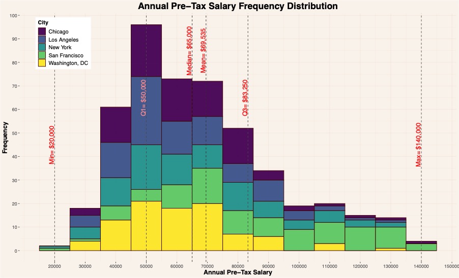
Graph 1: Frequency Graph for Pre-Tax Salaries across all 5 cities. Frequency is clustered in bin widths of US$10,000.
Within these five cities 20% of entry level professionals earned between $45,0001 and $55,000 in pre-tax salary. Similarly, entry level professionals in New York City, Los Angeles, and Chicago are most likely to earn within this range, whereas in San Francisco and Washington, DC can expect to earn between $65,001 and $75,000. The mean salary of the 480 entry level professionals is $69,535, with 68% earning between $44,311 and $94,759.
Estimating Post-Tax Salary
The post-tax salary is the amount a person has to live on, and so it is important to understand what percentage of the offered pre-tax salary it is. In the United States there are 4 main types of income tax 4,5: federal, state, city, and FICA. Excluding FICA, each has varying tax brackets that are calculated marginally based on pre-tax salary. This makes it difficult for someone to quickly understand what their post-tax salary is when offered a compensation package. Using Simple Linear Regression, a much easier method can be created to estimate post-tax salaries.
Graph 2 depicts trend lines for pre-tax and post-tax salaries and their relation to one another (salaries were placed in ascending order and plotted in that order on the x-axis). The post-tax salary one can expect to earn is directly under the pre-tax salary offered. Total income tax does not increase linearly - the graph displays a widening gap between the two trend lines. That is, as salary increases the greater the percentage of one's salary will be paid in taxes.
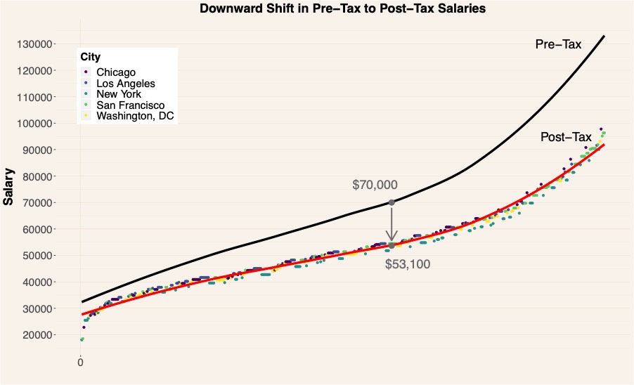
Graph 2: Displays the shift from a Pre-Tax to Post-Tax Salary. A Pre-Tax salary of $70,000 is closer to $53,100 after taxes
Correlation
The correlation between pre-tax and post-tax salary is 0.9973572. Due to the dependent nature of post-tax salaries on income this high positive correlation is expected.
Simple Linear Regression
As there was only one predictor variable a simple linear regression model was generated to estimate post-tax salaries.
Let x denote Pre-Tax Salaries, where x \(\geq\) annual minimum wage
\(\hat y\) represents the estimated post-tax salary
\(\hat y = 9029.9211 + 0.6315x\)
Therefore, a simplified method for estimating post-tax salary is to take 63% of the offered salary + $9,000. For example, if Pre-Tax Salary = $150,000, then \(\hat y\)= 9000+ (0.63 *150000) = $103,755.
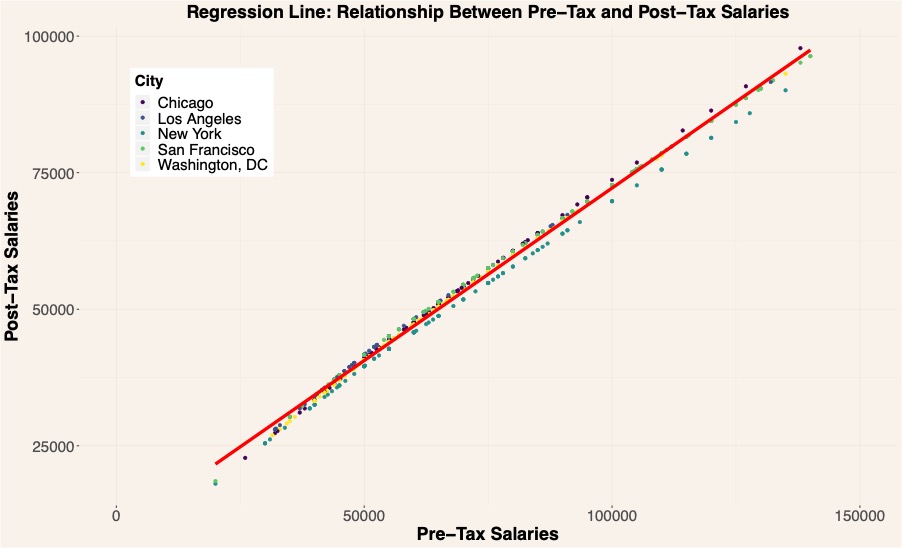
Graph 4: Regression Model and the Relationship Between Pre-Tax and Post-Tax Salaries
| Parameter | F(1,478) | Prob < F | R2 |
|---|---|---|---|
| Value | 9.007e+04 | 2.2e-16 | 0.9947 |
The large F-value and near zero P-value indicate that there is a relationship between post-tax salaries and pre-tax salaries - it rejects \(H_0: \beta_1 =0\) and accepts \(H_1: \beta_1 \neq 0\). Furthermore, R2= 0.9947 points out that approximately 99.47% of the variance found in post-tax salaries is explained by the predictor: pre-tax salaries.
| Parameter | Estimate | St. Error | T-Value | P(<|t|) |
|---|---|---|---|---|
| Intercept | 9029.9211 | 155.6 | 58.02 | < 2e-16 |
| Pre-Tax(x) | 0.6315 | 0.002104 | 300.12 | < 2e-16 |
While F-Value, P-Value and R2 provide insight into the entire model, each predictor variable is also analyzed independently to have a better understanding of the effect each predictor has on the outcome. In this case, there is only one predictor variable and so if the overall model is a strong fit so is the one variable: pre-tax salaries. The standard error tells us that on average there is a 0.2% error, so on average we should calculate between 63.336% to 62.9396% (which rounds to 63%).
| Parameter | SST | SSE | SSR |
|---|---|---|---|
| Value | 122,185,618,259 | 121,540,637,938 | 644,980,321 |
Due to the large sample size and their range of values the variability represented in SST, SSE and SSR do not necessarily represent inaccuracy. From R2 99.47% of the variability has already been accounted for. Analyzing the mean standard error and residual values give a much better perspective of the errors and their variability with respect to the linear model.
The mean squared error between a predicted post-tax salary and actual post-tax salary is $1,162, meaning that on average the standard error between the two values is approximately ± $34.09. To further analyse and understand the suitability of the regression model, the residual values between the sample mean of post-tax salaries and actual post-tax salaries within the sample set were plotted in Graph 5. Four distinct patterns can be spotted for each state with its own tax brackets: California (San Francisco & Los Angeles), Illinois (Chicago), New York (New York City), and Washington, DC. Unsurprisingly, the patterns within the residual plot indicate 1) a non-linear model may be more suitable and 2) each state should be modelled individually. Not only would modelling each state's taxes individually produce better results, but it makes more sense considering that a person only pays income tax for one state for a specific portion of their salary.
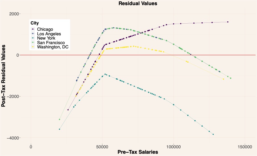
Graph 5: Plot of Residual Values Between Sample Mean of Post-Tax Salaries and Actual Post-Tax Salaries
Summary
Taxes increase marginally and each state has its own set of tax brackets. Clustering sample data from 5 cities in 4 states still produced a regression model which estimated post-tax salaries with a low root mean squared error. The high correlation (0.9973572) between pre-tax salaries and post-tax salaries reveals that even though different states have different tax brackets, they are still similar. Due to the non-linearity of tax brackets a non-linear model and each state being modelled individually would have probably produced better estimates.
What Proportion Can Expect to Earn Above Cost of Living?
A new graduate is considered to be able to afford cost of living in their city if annual post-tax salary > average cost of living. Of the 480 salary records within the sample set, 424 received a salary that afforded the person the cost of living within the city they lived in. A 2-tailed Confidence Interval test at 90% confidence level was calculated to have a clearer understanding of which proportion of new graduates can afford cost of living. Because it is unknown if there are false salary records in the sample set, only 90% of the results are estimated to represent the population's results.
Let N =480
\(\hat p = 424/480= ~0.675\)
Confidence interval at 90%, 2-tailed z-test= 1.6449
\(z= \sqrt{(0.675 * (1-0.675))/480} \)
\(0.675 \pm 1.6449 * z\)
\((0.6398349, 0. 7101651)\)
With 90% confidence it can be said the proportion of the population earning above the average cost of living in one of the 5 cities is between 64% and 71%, where the population represents students about to enter the work force.
Is there an equal chance in each city?
Cost of living varies from city to city, the highest being San Francisco at $56,724 and the lowest Chicago, at $31,872 - a $24,842 difference. The theory that new graduates have the same likelihood of earning above cost of living from city to city was tested using a one-way ANOVA test and hypothesis test. The data used for this test was Extra = Post-Tax Salary- Cost of Living.
Let x= Extra
If \(\bar{x} \geq\) 0, avg salary is > cost of living
If \(\bar{x}\) < 0, avg salary is < cost of living
\(H_0: \bar x_i = \bar x_j\)
\(H_1: \bar x_i \leq \bar x_j\)
Where i,j = New York City, Los Angeles, San Francisco, Chicago, and Washington, DC
F = 24.48 > f.05 (4,475)= 0.000 at the significance level of 0.05, therefore we reject H0; entry level graduates do not have an equal chance of earning above the average cost of living across all cities. On average, new graduates will earn $17,620 above the cost of living in Chicago, $12,474 in Washington, $10,903 in San Francisco, $8,169 in Los Angeles, and -$4,683 in New York City.
The graph below segments post-tax salaries by city, and the average cost of living index was placed relative to the proportions of the sample set that earns pre-tax salaries above and below it. From this sample set Chicago appears to be the most affordable and New York City the least affordable - this follows that of these 5 cities New York City is ranked highest and Chicago lowest on the Cost of Living Index.
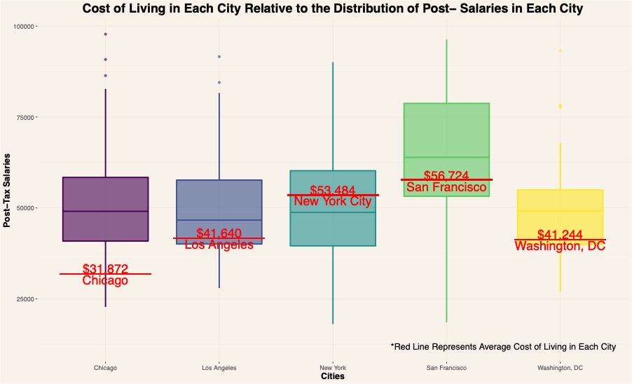
Graph 6: Cost of Living in Each City Relative to the Distribution of Post- Salaries in Each City
Conclusion
Salaries offered are often influenced by degree, industry, job title, location and many other factors. Even though
all records within this sample set are for entry level professionals, each may be entering the work force with their own unique
background. As such, a wide range of salaries is offered. Based on this sample set, approximately two-thirds of entry level
professionals can expect to earn above the average cost of living in New York City, Los Angeles, San Francisco, Chicago and
Washington, DC with an annual pre-tax salary between $45,001 and $55,000. Using the regression model: \(\hat y\) = 9029.9211 + 0.6315x
the respective estimated post-tax salary is between $37,350 and $43,650. Unfortunately for those choosing to move to New York City,
their chance of earning above the average cost of living is much lower than those who move to Chicago - 95% of new graduates in
Chicago earned above average cost of living, 72% in Los Angeles, 66% in Washington DC, 63% in San Francisco, and 41% in New York
City. The data within this sample set is crowdsourced and therefore there is room for error in the data set. The distribution of
industries is 1) heavily weighted towards the technology industry, 2) greatly differed across each city, for example: NYC is ~30%
tech salaries and SF ~70%. In the United States the technology industry is known for paying salaries higher than other industries.
All in all,
Appendix
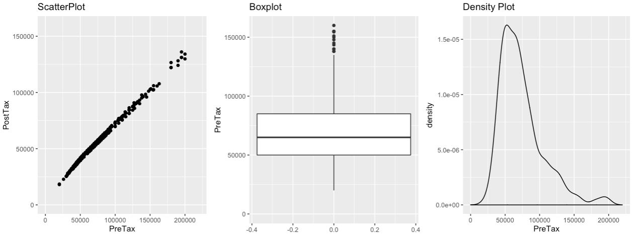
A1: Inital Sample Set Plotted
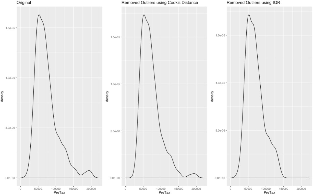
A2: Comparison of density plots before and after removing outliers
Bibliography/Citations
- Author: WSJ.com Graphics
Article title: Where Graduates Move After College
Website title: WSJ
URL: https://www.wsj.com/graphics/where-graduates-move-after-college/ - Author: Cost of Living
Article title: Cost of Living Index. Updated Feb 2020
Website title: Expatistan, cost of living comparisons
URL: https://www.expatistan.com/cost-of-living/index - Author: Comparably - Transparent Compensation & Culture
Website title: Comparably
URL: https://www.comparably.com/ - Author: Tina Orem
Article title: 2019-2020 Federal Income Tax Brackets and Tax Rates - NerdWallet
Website title: NerdWallet
URL: https://www.nerdwallet.com/blog/taxes/federal-income-tax-brackets/ - Article title: California Income Tax Calculator - SmartAsset
Website title: SmartAsset
URL:https://smartasset.com/taxes/california-tax-calculator
Comments About Data
The salary data was acquired from Comparably.com3. Comparably mostly focuses on the technology industry, and it is reflected in the salary records. The data is crowdsourced and therefore there is room for error in the data (i.e. the record could be false). In the United States the technology industry is known for paying salaries higher than other industries - this means the sample set may inflate results.
The distribution of industries within each city differs greatly, and so these variations will also be reflected in the data (for example, NYC is ~30% tech salaries and SF ~70%).
In addition, each entry level professional may have their own unique background contributing to the large range in entry level salaries. These include past summer internships, a Master's degree vs a Bachelor's degree, the field of study, etc.
In the United States there are many deductions (for example: student loans, mortgage loans, number of dependents, etc.) that can be applied to reduce taxable income, but for this study a homogenous approach was taken and only the standard deduction of $12,200 USD was deducted.