Case Study: Optimising Fuel Flow for the Falcon Heavy During First Stage Burn
Problem Brief
The Falcon Heavy launch vehicle, designed to carry humans into space, does not reach the height necessary for successful operations. Preliminary analysis has indicated that the issue stems from an underperforming first stage, more precisely from a suboptimal flow of fuel into the combustion chamber of the rocket engine. You are tasked with optimising the fuel flow in order to maximise the height of the rocket at the end of the first stage burn.
Solution Report
Model was coded using AMPL.
Introduction
The Falcon Heavy rocket ship is being designed by SpaceX with the purpose of shuttling humans into space. Unfortunately it is not ready for its maiden voyage due to complications. During testing it was found that the rocket cannot achieve the height needed to become a successful mission. Upon further investigation it was discovered that the first stage burn is performing sub-optimally because of the fuel flow into the rocket engine's combustion chamber.
The affects of fuel flow on the maximum height of the rocket at the end of first stage burn can be understood by evaluating the following variables as they transition through time:
height: [t0, tfinal] -> R
velocity: [t0, tfinal] -> R
mass: [t=0, tfinal] -> R
To do so, the first derivative of each is calculated. From equation (1) height increases proportionally with velocity as time increases. (2) is acceleration at time t, and mass (3) is negatively proportional to thrust at time t. Lastly drag/friction is also relative to time, velocity and height:
\(h'(t) = v(t)\))(1)
\(v'(t) = {\theta(t)- D(h(t),v(t)\over m(t)}- ({h(0)\over h(t)})^2\)(2)
\(m'(t) = -2\theta(t)\)(3)
\(D(h(t),v(t)) := D_0 \times (v(t))^2 \times exp(-h_0 {h(t)-h(0)\over h(0)})\)(4)
Where 't' is any given time within \([t_0, t_{final}]\). The rocket begins take off at t0 and will finish firing at \(t_{final}\).
Ideally, there will only be a global solution (not multiple local optimal points), so using the second derivative convexity is tested. It can quickly be seen that m''(t)<0 inferring that the problem is non-convex.
Formulation of Model
As tfinal is unknown, there is no upper constraint on time and it is essentially infinite. This lack of boundary adds to the difficulties of finding an optimum solution as there are now also infinite decision variables. To overcome this, time is discretised into intervals using a parameter N, where ti = i/N * tfinal, for i= 0..N and tfinal = tN.
Another adjustment that will lessen the computational strain, the aforementioned functions (1-3) are converted into finite difference equations using numerical differentiation. The step lengths will be dictated by tfinal/N and will therefore change depending on N and tfinal. These transformations convert the problem into a nonlinear optimisation problem.
Velocity: \(\overline v_k\) = velocity at kth time step for k=0..N
Height: \(\overline h_k\) = height at kth time step for k=0..N
Mass: \(\overline m_k\) = mass at kth time step for k=0..N
Thrust: \(\overline \theta_k\) = thrust at kth time step for k=0..N
Friction: \(D(\overline h_k,\overline v_k)\) = friction with the atmosphere in relative to height and velocity of the rocket at time t
tfinal: the time at the end of max height
N: the number of steps in time
\(\max\limits_{t_{final} \in \rm I\!R^N \overline h, \overline v, \overline m, \overline \theta \in \rm I\!R^{N+1} }\) \(\overline h_N\)
subject to: \(\qquad\) \(N(\overline h_1 - \overline h_0) = t_{final} \times \overline v_0\)(5)
\(N(\overline h_{k+1} - \overline h_{k-1}) = 2t_{final} \times \overline v_k\)(6)
\(N(\overline h_N - \overline h_{N-1} = t_{final} \times \overline v_N\)(7)
\(N(\overline v_1 -\overline v_0) = t_{final} ( {\theta_0 - D(\overline h_0, \overline v_0) \over \overline m_0} - ({h(0)\over h_0})^2)\)(8)
\(N(\overline v_{k+1} -\overline v_{k-1}) = 2t_{final} ( {\theta_k - D(\overline h_k, \overline v_k) \over \overline m_k} - ({h(0)\over h_k})^2)\)(9)
\(N(\overline v_N -\overline v_{N-1}) = t_{final} ( {\theta_N - D(\overline h_N, \overline v_N) \over \overline m_N} - ({h(0)\over h_N})^2)\)(10)
\(N(\overline m_1 - \overline m_0) = t_{final} \times (-2\theta_0)\)(11)
\(N(\overline m_{k+1} - \overline m_{k-1}) = 2t_{final} \times (-2\theta_k)\)(12)
\(N(\overline m_N - \overline m_{N-1}) = t_{final} \times (-2\theta_N)\)(13)
\(D(\overline h, \overline v) = D_0 \times (\overline v)^2 \times exp(-h_0 {\overline h_k- h(0) \over h(0)})\)(14)
\(v(0) = 0\)(15)
\(h(0) = 1\)(16)
\(m(0) = 1\)(17)
\(m(t_{final}) = 0.6\)(18)
\(v(t) \geq 0\)(19)
\(h(t) \geq h(0)\)(20)
\(m(t_{final}) \leq m(t) \leq m(0)\)(21)
\(0\leq \theta(t) \leq \theta_{max}\)(22)
Constant Parameters:\(\quad \theta_{max} := 3.5\)
\(h_0 := 500\)
\(v_0 := 620\)
\(D_0 := v_0/2\)
The following equations are also used as initial conditions:
\(Velocity: v(t) = ({t \over t_{final}})(1-{t \over t_{final}})\)(23)
\(Mass:m(t)= 1+({t \over t_{final}})(0.6-1)\)(24)
Equation (18) states that the mass of the rocket at tfinal is 0.6, this is because 0.4 of the mass is fuel. The discretisation of time has led to 4N decision variables, where N = 50, 100, 200 or 400. There are a total of 14 constraints, with equations (8), (9), (10), and (11) being nonlinear.
Assumptions
- The rocket can continue rising after all fuel has been consumed by using the residual momentum to achieve a maximum height.
- The rocket's direction and path is always straight upward.
- Thrust is linearly proportional to fuel burned, therefore the engine burns fuel equally efficiently regardless of fuel burn rate.
- By taking educated guesses at setting parameter N, an appropriate step length can be found and will accurately depict the maximum height.
- Though the solution found is a local maximum, there's hope it is also the global maximum.
Brief Description On How It's Solved
Four different solvers are used within AMPL: LOQO, SNOPT, KNITRO, and MINOS. Each is known for its ability to solve local maxima/minima in nonlinear, non-convex optimisation problems.
To initialise the model given starting points are inputted: \(t_{final}=1, \overline h_k=1, \overline \theta_k= \theta_{max}/2\), and the values N = 50, 100, 200, 400 are tested. Between the combinations of solvers and parameter N, there are 16 trials within the first round of testing.
Additionally, using a quadratic equation to describe the starting point of \(v(t)\) is the simplest polynomial order that can be used to represent the expected behaviour of velocity at times \(v(t=0)=0\) and \(v(t=t_{final})=0\), with there being a peak at step \(t=k\)could be 1,..., N-1). Therefore the given initial condition seems suitable and does not need to be changed. The starting point for mass, \(m(t)= 1+({t \over t_{final}})(0.6-1)\) indicates that mass burn is linear with time and ranges between 1 to 0.6.
Because the problem is non-convex, the starting points matter. A second round of 16 trials is then tested using the starting point \(t_{final}= 0.5\). All other starting points, N values and solvers from the first round are kept the same.
Data associated with time, velocity, height, mass and thrust are documented at each step for all trials. An emerging pattern demonstrated that trails with more steps (and shorter step lengths) had better results when using solvers SNOPT and KNITRO. This led to testing other combinations of starting points where \(\overline h_k=0.5\) and \(\overline \theta_k= \theta_{max}\). Other random starting points were tested, but results were never improved using them (so it seemed unnecessary to document them).
As the output of the objective will need to be rescaled to know the true height, the stopping criteria is set to 9 digits of accuracy: ε ≤ .1e-8 between the two highest heights. To analyse results data within each table were reviewed and various combinations of decision variables were plotted on 2D graphs.
Results
Results for 16 Initial Trials
When parameter N used higher values, \(\overline h_k\) was more likely to achieve greater heights for all solvers except for MINOS (which performed worse as N increased). For all 16 trials, the predictor variable 'Thrust' was plotted against the response variable 'Height'. Visualising the data uncovered three phases, and two main types of patterns of fuel flow. Trials 7 (Figure 1) and 12 (Figure 2) are examples of the patterns (refer to table A1 to see starting points and solvers used) .
During the second phase of the burn, trial 12 displays a zig-zagging pattern between maximum and zero fuel burn. Trial 7 has a more stable second phase where fuel burn gradually increases. When comparing the two types of patterns there was no identifiable trend in which performed better. Lastly, height differs by 0.001438158 units between the highest and lowest heights; that is Trial 3's max height is 11.2038% (to 4dp) less than Trial 12's.
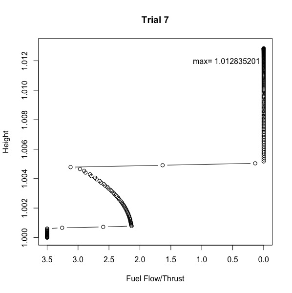
Figure 1: Trial 7, Height vs Fuel Flow/Thrust
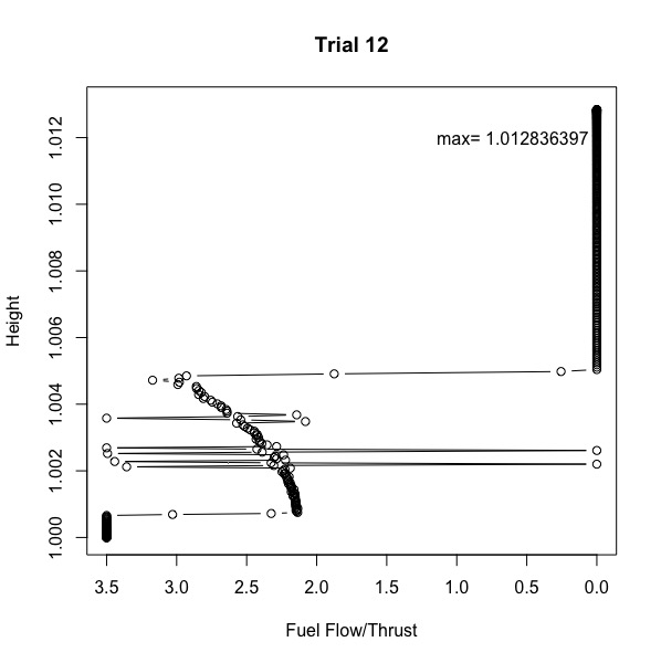
Figure 2: Trial 12, Height vs Fuel Flow/Thrust
A total of 43 trials were computed. The results from the top 5 performing (by height) can be seen in Table 1 below, and the results from all in Table A1.
Observation From All Trials
Height does not increase linearly with time, and smaller step sizes \((t_{final}/N)\) generally lead to a better outcome. Since the starting points are important to finding a local maxima, various were tested. Initiating \(\theta\) at \(\theta_{max}\) had the most impact on increasing height, whereas \(t_{final}\) and \(\overline h_k\) did not improve the objective function as much (can be seen in rows 2 to 4 of Table 1). Table 1's results show that the combination of starting points for trial 39 has highest max \(\overline h_k\).
Table 1: Results from top 5 outcomes (heights)
| Trial No. | Solver | N | \(t_{final}\) | \(\overline h_k\) | \(\overline \theta_k\) | max \(\overline h_k\) | \(k\) |
|---|---|---|---|---|---|---|---|
| 39 | SNOPT | 400 | 0.5 | 0.5 | 3.5 | 1.012836497 | 0,...,N |
| 37 | SNOPT | 400 | 1 | 0.5 | 3.5 | 1.012836496 | 1,...,N-1 |
| 38 | SNOPT | 400 | 0.5 | 0.5 | 3.5 | 1.012836496 | 1,...,N-1 |
| 43 | SNOPT | 400 | 0.25 | 0.5 | 3.5 | 1.012836496 | 1,...,N-1 |
| 41 | KNITRO | 400 | 1 | 0.5 | 3.5 | 1.012836468 | 1,...,N-1 |
Results from Trial 39
The rate of fuel flow can be observed in 3 main stages:
- The rocket takes off a full throttle (max fuel flow) to get off the ground, thrust is constant and velocity is quickly picking up during this period.
- The fuel flow is optimised to overcome the increase in drag due to increasing velocity and height. Fuel flow drops significantly to ≈2.1 and gradually increases to 3.1 within 0.5 time units. Increase in velocity slows down a bit during this initial transition, then ramps up until the fuel is finished.
- The rocket continues to rise while decelerating due to drag, which continues for 63.25% of steps.
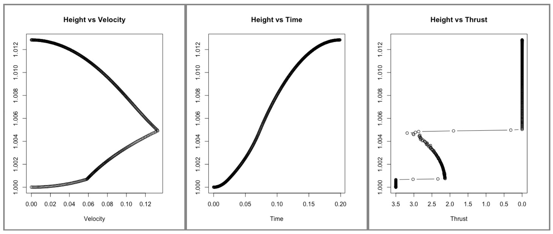
Figure 3 (L to R): Height vs Velocity for Trial 39 | Figure 4: Height vs Time for Trial 39 | Figure 5: Height vs Thrust for Trial 39
Actionable Recommendations
- Because the problem is non convex, the solution found is a local maxima and not necessarily a global maximia, research should be done to confirm that it is a viable solution to the problem.
- Testing a wider range of solvers, and values for parameter N
- Is max thrust limited by physical infrastructure? The rate of fuel flow, especially within the first phase of take off is important to achieving a maximum heigh, experimentation should be done with a max thrust > 3.5
- Within this model throttle was able to change infinitely, but real engines do not respond that way. Additional constraints should be added for the max change in throttle between time steps.
Suggestions for Further Investigations
- It was previously mentioned that fuel burn performs linearly to thrust, but engines are more likely to have non-linear relationship between thrust and fuel burn rate. Further test should be carried out to understand how the engine performs then rewrite the formula to more accurately predict how it performs.
- Though recommended action #2 is testing different values of N, consideration must be taken to ensure that the step length is not too small or too large as they can cause zero values within the finite differences calculations or the estimate of the slope of the tangent may be less accurate.
- The computational time of this model was rather short, meaning that a more robust model that may need more computational time and power can be used to estimate height
Appendix
Table A1: Trials and their outcomes
| Trial No. | Solver | N | \(t_{final}\) | \(\overline h_k\) | \(\overline \theta_k\) | max \(\overline h_k\) | \(k\) |
|---|---|---|---|---|---|---|---|
| 1 | MINOS | 50 | 1 | 1 | 1.75 | 1.012809645 | 1,...,N-1 |
| 2 | MINOS | 100 | 1 | 1 | 1.75 | 1.012830166 | 1,...,N-1 |
| 3 | MINOS | 200 | 1 | 1 | 1.75 | 1.011398239 | 1,...,N-1 |
| 4 | MINOS | 400 | 1 | 1 | 1.75 | 1.011886695 | 1,...,N-1 |
| 5 | KNITRO | 50 | 1 | 1 | 1.75 | 1.012809643 | 0,...,N |
| 6 | KNITRO | 100 | 1 | 1 | 1.75 | 1.012830154 | 0,...,N |
| 7 | KNITRO | 200 | 1 | 1 | 1.75 | 1.012835201 | 0,...,N |
| 8 | KNITRO | 400 | 1 | 1 | 1.75 | 1.012836341 | 0,...,N |
| 9 | SNOPT | 50 | 1 | 1 | 1.75 | 1.012809645 | 1,...,N-1 |
| 10 | SNOPT | 100 | 1 | 1 | 1.75 | 1.012830162 | 1,...,N-1 |
| 11 | SNOPT | 200 | 1 | 1 | 1.75 | 1.012829353 | 1,...,N-1 |
| 12 | SNOPT | 400 | 1 | 1 | 1.75 | 1.012836397 | 1,...,N-1 |
| 13 | LOQO | 50 | 1 | 1 | 1.75 | 1.012809645 | 0,...,N |
| 14 | LOQO | 100 | 1 | 1 | 1.75 | 1.012830161 | 0,...,N |
| 15 | LOQO | 200 | 1 | 1 | 1.75 | 1.012835188 | 0,...,N |
| 16 | LOQO | 400 | 1 | 1 | 1.75 | 1.012835551 | 0,...,N |
| 17 | MINOS | 50 | 0.5 | 1 | 1.75 | 1.012809645 | 1,...,N-1 |
| 18 | MINOS | 100 | 0.5 | 1 | 1.75 | 1.012830166 | 1,...,N-1 |
| 19 | MINOS | 200 | 0.5 | 1 | 1.75 | 1.011398239 | 1,...,N-1 |
| 20 | MINOS | 400 | 0.5 | 1 | 1.75 | 1.011886695 | 1,...,N-1 |
| 21 | KNITRO | 50 | 0.5 | 1 | 1.75 | 1.012809623 | 0,...,N |
| 22 | KNITRO | 100 | 0.5 | 1 | 1.75 | 1.012830019 | 0,...,N |
| 23 | KNITRO | 200 | 0.5 | 1 | 1.75 | 1.012835199 | 0,...,N |
| 24 | KNITRO | 400 | 0.5 | 1 | 1.75 | 1.012836405 | 0,...,N |
| 25 | SNOPT | 50 | 0.5 | 1 | 1.75 | 1.012809645 | 1,...,N-1 |
| 26 | SNOPT | 100 | 0.5 | 1 | 1.75 | 1.012830163 | 1,...,N-1 |
| 27 | SNOPT | 200 | 0.5 | 1 | 1.75 | 1.012826693 | 1,...,N-1 |
| 28 | SNOPT | 400 | 0.5 | 1 | 1.75 | 1.012836397 | 1,...,N-1 |
| 29 | LOQO | 50 | 0.5 | 1 | 1.75 | 1.012809645 | 0,...,N |
| 30 | LOQO | 100 | 0.5 | 1 | 1.75 | 1.012830165 | 0,...,N |
| 31 | LOQO | 200 | 0.5 | 1 | 1.75 | 1.012835121 | 0,...,N |
| 32 | LOQO | 400 | 0.5 | 1 | 1.75 | 1.012835121 | 0,...,N |
| 33 | KNITRO | 200 | 1 | 0.5 | 1.75 | 1.012835156 | 1,...,N-1 |
| 34 | KNITRO | 400 | 1 | 0.5 | 1.75 | 1.012836265 | 1,...,N-1 |
| 35 | SNOPT | 200 | 1 | 0.5 | 1.75 | 1.012829353 | 1,...,N-1 |
| 36 | SNOPT | 400 | 1 | 0.5 | 1.75 | 1.012836397 | 1,...,N-1 |
| 37 | SNOPT | 400 | 1 | 0.5 | 3.5 | 1.012836496 | 1,...,N-1 |
| 38 | SNOPT | 400 | 0.5 | 0.5 | 3.5 | 1.012836496 | 1,...,N-1 |
| 39 | SNOPT | 400 | 0.5 | 0.5 | 3.5 | 1.012836497 | 0,...,N |
| 40 | MINOS | 400 | 0.5 | 0.5 | 3.5 | 1.011421983 | 0,...,N |
| 41 | KNITRO | 400 | 1 | 0.5 | 3.5 | 1.012836468 | 1,...,N-1 |
| 42 | KNITRO | 400 | 0.5 | 0.5 | 3.5 | 1.012836381 | 1,...,N-1 |
| 43 | SNOPT | 400 | 0.25 | 0.5 | 3.5 | 1.012836496 | 1,...,N-1 |
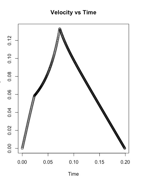
Figure A1: Velocity vs Time for Trial 39
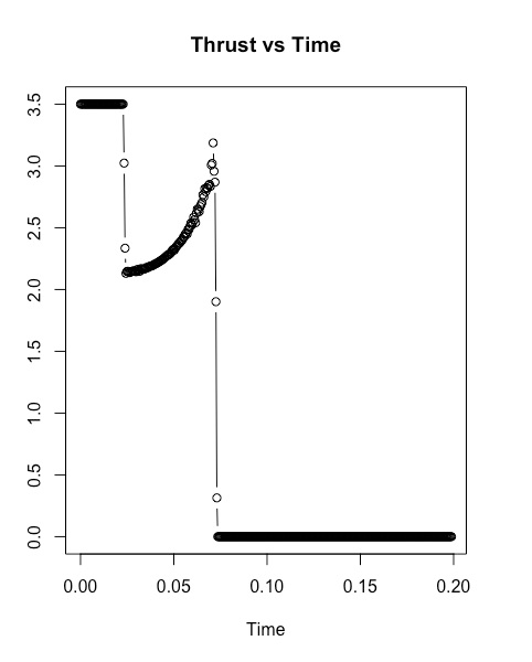
Figure A2: Thrust vs Time for Trial 39