ORANGE JUICE PRODUCTION PLANNING USING LINEAR PROGRAMMING
Problem Brief
You have been assigned to provide analytics experience to the company UniCitrus. UniCitrus is a major producer of frozen concentrated orange juice in Brazil. Three orange varieties are used: Hamlin, Pera, and Valence. The company buys the production from selected orange plantations, picks the fruits, processes it into juices, and blends them into two products called Standard and Dairy. The Standard juice is primarily used by beverage industries all over the world. The slightly more expensive Dairy has to satisfy certain conditions on flavour, acidity, and colour, among others. The planning horizon is 3 months. Tasks to be completed:
- Determine a production plan that maximises the company's net profit during the planing horizon. Juice inventories are negligible at the beginning go the planning horizon.
- Capacity limitations of the juice plant were ignored in part 1; revise the model to take into account the following capacity constraints. The equipment at the plant can process 0.5 million boxes of Pera oranges per month if this is the only variety processed. Hamlin oranges use 10% more capacity, and Valencia oranges use 10% less capacity. The effective plant capacity will therefore depend on the proportions of the different varieties processed.
- Orange growers in northern Brazil produce a lot of Valencia oranges. A truckload of Valencia oranges consists of 1000 boxes. Let \(\lambda\) denote the cost for purchasing and transporting a truckload of oranges from the north to the juice plant. Evaluate the effects of increasing the availability of Valencia oranges on the optimal production plant, treating \(\lambda\) as the optimal parameter.
Report
The model was built and solved using Xpress IVE.
Introduction
UniCitrus, a producer of frozen concentrated orange juice in Brazil, has requested a predictive analysis of the maximum net profit they can earn during a 3 month planning horizon. UniCitrus has provided the demand they have projected for the two juice types they produce, Standard and Dairy, in Table 1, as well as each juice's selling price. If demand is fully met, there is the potential to earn £3,140,000 in revenue (even though UniCitrus has stated that it is not necessary for all demand to be met). To produce the two juice types UniCitrus uses 3 varieties of oranges - Hamlin, Pera, and Valencia; the current expected availability (supply) is listed in Table 2. The cost to purchase and transport each box of oranges is £1. However, each box of orange variety has a different weight, so the cost per tonne for each variety differs with Pera costing £270.27/tonne, then Hamlin at £285.71/tonne, and Valencia at £294.18/tonne
Table 1: Demand (in Tonnes) & Selling Price per Tonne
| Product | Month 1 | Month 2 | Month 3 | Selling Price/Tonne |
|---|---|---|---|---|
| Standard | 500 | 1500 | 700 | £1,000 |
| Dairy | 200 | 1500 | 100 | £1,100 |
Table 2: Expected Availability/Supply in Tonnes
| Month | Hamlin | Pera | Valencia |
|---|---|---|---|
| 1 | 1050 | 925 | 0 |
| 2 | 1225 | 295 | 170 |
| 3 | 350 | 1850 | 340 |
Additionally, the cost to run the juice plant each month is fixed at £500,000, and storing juice inventory is £10/tonne/month. Standard and Dairy juice are produced by using different percentage combinations of the 3 different orange varieties. During each batch of production, this combination can change (as it is affected by supply) as long the criteria in Table 3 is met.
Table 3: Percentage of Juice Variety in Each Product
| Standard | Dairy |
|---|---|
| 0 \(\leq\) Hamlin \(\leq\) 0.25 | 0 \(\leq\) Hamlin \(\leq\) 0.3 |
| 0.6 \(\leq\) Pera \(\leq\) 1 | 0.5 \(\leq\) Pera \(\leq\) 1 |
| 0 \(\leq\) Valenica \(\leq\) 0.4 | 0.15 \(\leq\) Valenica \(\leq\) 0.5 |
Formulation of Model
Months: m= 1, 2, 3
Orange Variety: o= 1, 2, 3
Juice Type: j= 1, 2, 3
Let: s= supply
d= demand
x= juice sold to meet month's demand (in tonnes
y= oranges purchased and produced into juice within the month (in tonnes)
h= start of month inventory
i= end of month inventory
P = juice plant
Task 1- Base Model
Maximise: Net Profit= \( \sum_{m=1}^3\sum_{o=1}^3\sum_{j=1}^2 (x_{mj} \) \(\times SellingPrice - 10i_{moj})\) \(- (1000y_{moj}/ boxweight_o))\) \(- 500000\sum_{m=1}^3P_m\)
Subject to:
Supply: \(\sum_{j=1}^2 y_{moj} \leq s_{mo}\)
Demand: \(\sum_{j=1}^2 x_{moj} \leq d_{mj}\)
Inventory: for m= 1\(\quad x_{moj}- y_{moj} = i_{moj}\)
\(x_{moj} \leq y_{moj}\)
for m> 1 \(\quad y_{moj} + i_{(m-1)oj} = h_{moj}\)
\(i_{(m-1)oj} + y_{moj} - x_{moj} =\)\( i_{moj}\)
\(m_{moj} \leq h_{moj}\)
Mixtures:\(x_{moj} \geq \sum_{o=1}^3 minpercent_{oj} \times x_{moj}\)
\(x_{moj} \leq \sum_{o=1}^3 maxpercent_{oj} \times x_{moj}\)
\(y_{moj} \geq \sum_{o=1}^3 minpercent_{oj} \times y_{moj}\)
\(y_{moj} \leq \sum_{o=1}^3 maxpercent_{oj} \times y_{moj}\)
Purchasing in thousands: \(\quad \sum_{o=1}^3 y_{moj} / boxweight_o= box\_const_{mo}\)
** \(box\_const_{mo}\) is an integer
Task 2- Capacity Limitations
Total Capacity: \(\quad \sum_{j=1}^2 (\frac {y_{m1j}} {1575} + \frac {y_{m2j}} {1850} + \frac {y_{m3j}} {1870}) \leq 1\)
Task 3- New source available for Valencia Oranges
The updates made throughout the model to adjust for the new source of Valencia oranges are in black, while the elements that already existed are in gray.
1. Orange Variety: o= 1, 2, 3, 4
2. Supply matrix
[1050, 925, 0, 10000
1225, 925, 170, 10000
350, 1850, 340, 10000]
3. New expense to subtract from Net Profit
Net Profit= \(\sum_{m=1}^3\sum_{o=1}^4\sum_{j=1}^2 ( x_{mj} \times SellingPrice\) \(- 10i_{moj})\)
\(- 1000 \sum_{m=1}^3\sum_{o=1}^3\sum_{j=1}^2 (y_{moj}/boxweight_o)\)
\(- 500000 \sum_{m=1}^3P_m\)
\(- \lambda\sum_{m=1}^3\sum_{j=1}^2 (y_{m4j}/boxweight_o)\)
4. Update mixture constraints: for orange variety o>2
\(x_{m3j} + x_{m4j} \geq \sum_{o=1}^3 minpercent_{3j} \times x_{moj}\)
\(x_{m3j} + x_{m4j} \leq \sum_{o=1}^3 maxpercent_{3j} \times x_{moj}\)
\(y_{m3j} + y_{m4j} \geq \sum_{o=1}^3 minpercent_{3j} \times y_{moj}\)
\(y_{m3j} + y_{m4j} \leq \sum_{o=1}^3 maxpercent_{3j} \times y_{moj}\)
5. Capacity
\(\sum_{j=1}^2 (\frac {y_{m1j}} {1575} + \frac {y_{m2j}} {1850} + \frac {y_{m3j}} {1870} + \) \(+ \frac {y_{m4j}}{1870}\) \() \leq 1\)
Assumptions
- Inventory is for juice (and not oranges), therefore any oranges purchased within a month must be processed into juice. Carry forward effect: oranges are purchased based on ratios needed for juice mixture constraints.
- Inventory is held for one month, i.e. if juice is produced in month 1 it must be sold either in month 1 or month 2.
- If there are any months during the manufacturing cycle in which there is no production, the plant does not need to run during this time. It is assumed if the plant is not in production the entire cost of £500,000 to run the plant does not need to be spent.
- Each orange variety is purchased per 1000 boxes.
- It was not specified what percentage of each orange will convert to juice during the production process, so we assume there is no loss in weight (i.e.f one tonne of an orange variety is purchased it will produce one tonne of juice).
- There is 0 waste.
- Contract for northern Brazilian Valencia oranges is a month-to-month contract, so UniCitrus is not bound to solely purchase their Valencia oranges from that one source every month.
- Northern Brazilian Valencia orange boxes weigh the same as the original Valencia orange boxes.
Solution Description
Task 1
To solve Task 1's objective function, 3 primary variables were established to calculate the optimum combination of juice in tonnes: i) x - juice sold to meet that month's demand ii) y - quantity of oranges converted into juice that month, and iii) i - portion of juice produced in advance and held in inventory to meet the following month's demand. To simplify calculations, all units were converted into tonnes to align with using 'juice sold in tonnes' in the revenue prediction. Additionally, a constraint was created for boxes to be purchased per thousand boxes (because it would be unlikely that a large-scale juice producer would purchase supply per box).
UniCitrus sells its products by the tonne, therefore within each batch of juice the mixed orange varieties used need not be an integer, but the summed values within the batch has to be a whole number (abiding by the no waste policy). Due to supply limitations of Valencia oranges it was clear from the start that it would not be possible to produce Dairy Juice in Month 1, and so meeting all demand was not a primary concern. Lastly, to optimize the use of the juice plant a supplementary goal of producing juice to meet demand in as few months as possible was implemented.
Task 2
Introduced a new constraint - production capacity for each orange variety. The capacity constraint needed to be accounted for both vertically (within each orange variety) and horizontally (across all varieties). Capacity constraints were converted into tonnes to match the metrics of the existing model.
Task 3
A new source for Valencia oranges became available, presenting the opportunity to meet all demand. Because purchasing and transportation cost \(\lambda\) is unknown, the two sources of Valencia oranges are treated independently within the supply matrix. Contrarily, the two sources are treated as one for mixture and processing constraints.
It is assumed that this new supply of Valencia oranges is bountiful and therefore a redundant constraint. Our new goal is to observe the effects of \(\lambda\) on maximising net profit. Though it is evident that net profit will attain maximum value when \(\lambda\)=0, we will scrutinize the relationship between net profit and \(\lambda\) as it increases.
Results
Task 1
The results from Task 1 demonstrated that the juice plant could meet the expected 3 months of demand within a 2-month production period with the current supply and mixture constraints, by utilizing inventory to save £488,620 (£500,000-£11,3880) from one less month of production. The net profit for Task 1 is £1,111,620.
Table 4: Juice Manufactured in Tonnes
| Month 1 | Month 2 | Month 3 | ||||
|---|---|---|---|---|---|---|
| Standard | Dairy | Standard | Dairy | Standard | Dairy | |
| Produced (y) | 938 | 0 | 1762 | 200 | 0 | 0 |
| Start Inventory (h) | 0 | 0 | 438 | 0 | 700 | 100 |
| Sold (x) | 500 | 0 | 1500 | 100 | 700 | 100 |
| End Inventory (i) | 438 | 0 | 700 | 100 | 0 | 0 |
Task 2
Thereafter, a processing capacity was introduced for each orange variety, limiting the quantity of juice that could be produced each month. This new constraint lowered net profit by 0.07% to £1,110,790. The quantity of juice processed in Task 1's Month 2 exceeded the processing capacity, and as a result shifted more of Month 2's demand to Month 1's production run. This consequently increased the amount of juice in inventory and decreased net profit. With this constraint we are still capable of meeting demand for the 3 months (with the exception of Dairy in Month 1) with only 2 months of production.
Table 5: Juice Manufactured in Tonnes
| Month 1 | Month 2 | Month 3 | ||||
|---|---|---|---|---|---|---|
| Standard | Dairy | Standard | Dairy | Standard | Dairy | |
| Produced (y) | 1121 | 0 | 1579 | 200 | 0 | 0 |
| Start Inventory (h) | 0 | 0 | 621 | 0 | 700 | 100 |
| Sold (x) | 500 | 0 | 1500 | 100 | 700 | 100 |
| End Inventory (i) | 621 | 0 | 700 | 100 | 0 | 0 |
Task 3
As expected, net profit (£1,632,400) is at its highest when \(\lambda\)=0, and decreases as \(\lambda\) increases. Graph 1 visualizes the effects of \(\lambda\) on net profit, and Table 6 summarizes net profit's gradual desensitization to \(\lambda\). When \(\lambda\) < 975, the northern Valencia oranges are the cheapest of all varieties available and are therefore the preferred supply, exposing net profit to become vulnerable to any \(\lambda\)'s movements so net profit is vulnerable to any changes in \(\lambda\). For every unit (one) \(\lambda\) changes (i.e. £ per truckload), net profit will alter by approximately £367.18. In contrast, when 975 £ \(\lambda\) < 19441 net profit will fluctuate by approximately £8.86 for each unit change in \(\lambda\). Lastly, when \(\lambda\) \(\geq\)19,441 it becomes fruitless to continue purchasing the new Valencia oranges, and so net profit plateaus and is now unaffected by any increases in \(\lambda\).
Table 6: Summary of the effects of \(\lambda\) on Net Profit
| \(\lambda\) | Impact |
|---|---|
| 0-974 | Net Profit is highly sensitive to \(\lambda\), within this range gradient= -367.18 |
| 975-19,440 | Net Profit is slightly sensitive to \(\lambda\), within this range gradient= -8.86 |
| 19,441+ | Net Profit will plateau at \(\lambda\)= 19,441 onward |
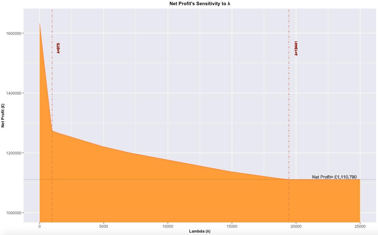
Graph 1: The Effects of \(\lambda\) on Net Profit
The introduction of \(\lambda\) has also impacted the purchasing distribution amongst the orange varieties. Graph 2 demonstrates the pivotal changes for quantities of northern Brazilian Valencia oranges purchased. In Month 1, UniCitrus does not have an alternative source of Valencia oranges; if they are to meet all demand, they must purchase oranges from the new source. Meanwhile in Month 2, there is an alternative option for Valencia oranges. These two cases provide enough information to understand the full effects of \(\lambda\) on purchasing distribution.
In Month 1, when \(\lambda\) < 919 it is more profitable to use the upper bound mixing percentage constraint for Valencia oranges in both juice types, because the new source of Valencia oranges is cheaper per tonne than any of the other varieties. Once \(\lambda\) exceeds 919 it becomes more expensive than purchasing Pera oranges, so we see the distribution shift towards the use of Pera oranges. Similarly, at \(\lambda\)=975, Hamlin oranges have a higher yield of weight/£ than Valencia oranges, further reducing the quantity of northern Valencia oranges purchased. Shortly after when \(\lambda\)=1000, both sources of Valencia oranges cost the same, therefore no preference is given to either source (since their effects on net profit are equivalent). Up until \(\lambda\)=1460 in Month 1, it is beneficial for UniCitrus to continue purchasing at least the minimum amount of Valencia oranges needed to meet all of Dairy demand. As \(\lambda\) increases past that amount, it is best for UniCitrus to continue purchasing Valencia oranges to meet a decreasing portion of Dairy demand. Lastly at \(\lambda\)= 19,441 Dairy production ceases as it is no longer profitable to purchase Valencia oranges
It is important to note that the purchasing decisions of orange varieties to maximize net profit is not solely dictated by their prices, but is also influenced by processing, mixing, and purchasing constraints.
Table 7: Summary of the Effects of \(\lambda\).
| \(\lambda\) | Impact |
|---|---|
| 0-918 | Purchase the max amount of Northern Brazil Valencia oranges to meet maximum mixture constraint. |
| 919-974 | Pera becomes the most cost-effective orange to purchase, but Northern Brazil Valencia oranges are still cheaper than hamlin. |
| 975-999 | Hamlin oranges are now better priced, and only what is needed of Northern Brazil Valencia oranges are purchased to meet full demand. |
| 1,000 | Both sources for Valencia oranges cost the same, and so no preference is given to either. |
| 1,001-1,459 | It is worthwhile to purchase the full amount of Brazilian Valencia oranges needed to fully meet demand if there are no alternatives. |
| 1,460+ | Only purchase as needed, and may not even meet full demand because it won't be the most profitable. |
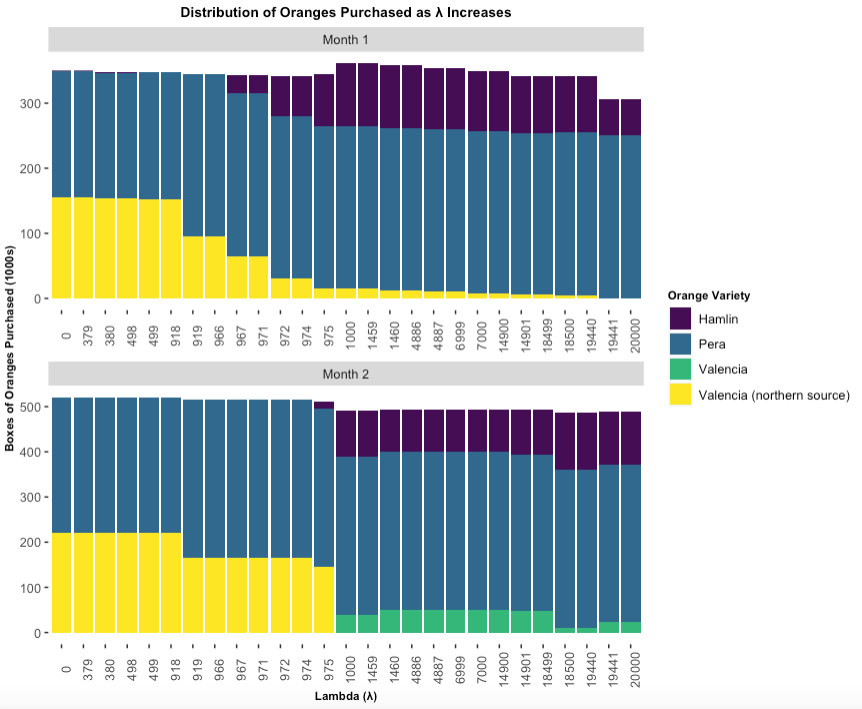
Graph 2: Boxes (in 1000's) of Oranges Purchased in Relation to \(\lambda\).
Recommendations
- Purchasing valencia oranges from the northern supplier will result in increased profits for UniCitrus if \(\lambda\) < 19441. UniCitrus should use Table A1 as a guideline for acceptable prices per truckload, and the identified number of truckloads that should be purchased at those prices.
- A more accurate prediction for Net Profit could be determined if UniCitrus segmented their monthly cost rather than presenting them in one lump sum (i.e. cost of running the juice plant at £500,000/month). In the model built, inventory replaces the need to run production every month, but it is unlikely that there would not be any expenses during those months. For example, members of the workforce will still need to be present to complete tasks such as managing inventory to meet demand.
- The supply of northern Brazilian Valencia oranges is bountiful, and can potentially supply enough oranges to meet demand for all 3 months of production. UniCitrus should utilize their current cost for Valencia oranges to leverage a lucrative deal with the new suppliers. If UniCitrus can negotiate for \(\lambda\) < 1000, then it would be sensible to purchase all Valencia oranges from the new supplier. But, if \(\lambda\) \(\geq\) 1000 UniCitrus should maintain their original source and only use the new Valencia if the initial supplier cannot meet their demands.
- Currently, Pera oranges are priced lowest per tonne, and Standard juice can be produced using only Pera oranges. If UniCitrus can source another supplier of Pera oranges who will charge the same or lower rate for Pera oranges, UniCitrus can increase net profit.
- If the juice plant is running it must perform at full capacity. This recommendation requires many other adjustments that need further investigation, such as increasing supply and demand, a longer inventory period and manufacturing cycle.
- If UniCitrus secures a contract for northern Brazilian Valencia oranges when \(\lambda\) < 919, then they should experiment with changing the mixture constraints to favour Valencia oranges. This will also maximise the amount of juice produced with current production capacity.
- Store inventory for oranges (not just juice). This way, excess supply can be stored for future demand, protecting UniCitrus from the case of, 'if a variety is not available one month and there was a high supply in previous months, and production capacity was met during those months it would still be possible to meet demand that would not have been otherwise met.'
Further Investigation
- In the current model, inventory is stored for one month. It would be prudent to learn (or for the analyst to be given access to such information) the shelf life of the juices, so that the model can be recreated to hold inventory for longer than a month or establish a steady inventory cycle.
- The 3-month planning horizon provided is insufficient for optimising the use of the juice plant. It would be better to analyse at least a year's worth of data to understand the ebbs and flows of supply and demand. This information will aid in planning what the length of the manufacturing cycle, inventory cycle, and ensuring production period operate at full capacity, which will further decrease cost/tonne of juice produced.
- UniCitrus should provide their past demand data, as it is possible that they are conservative in their demand projections. Because UniCiturs does not always operate at full capacity each month, the per tonne cost of production varies month to month. If is possible to increase demand it may be possible to lower and regulate the cost to produce each tonne by operating at full capacity during months of production.
- Assuming UniCitrus has been conservative while setting demand projections, and only produces juice to meet that demand, they are potentially losing out on higher revenue and profit. In this scenario the juice plant is not operating at full capacity, so we perform a cost benefit analysis of oversupply. The juice plant runs at a fixed cost each month, and so there is no variation in cost for running the plant at full capacity vs partial capacity. Therefore, if the factory is running at partial capacity and is increased to full capacity the only cost incurred would be cost to purchase and transport oranges and inventory. The average cost to purchase a tonne of oranges = £283.37, and the cost to inventory a tonne of juice each month= £10. Therefore, the average cost to oversupply is £283.37 + £10m (m for # of months stored), and the average to cost undersupply is £1050 - (£283.37 + £10m). Ultimately, it seems as though UniCitrus is losing more undersupplying.
Conclusion
In summary, it is profitable for UniCitrus to purchase the suggested quantity (can be found in Appendix: Table A1) of Valencia oranges from the new sources as long as \(\lambda\) < 19441. As depicted previously, there is an inverse relationship between the sensitivity of net profit and \(\lambda\), with there being two critical points segmenting net profit's sensitivity into thirds: \(\lambda\) < 975 is highly sensitive, 975 ≤ \(\lambda\)< 19441 is mildly sensitive, and \(\lambda\) \(\geq\) 19441 becomes immune. Likewise, major changes in purchasing distribution occur at the same values. Finally, if UniCitrus provides a breakdown of their expenses and historical supply and demand data a more accurate prediction for net profit can be modeled